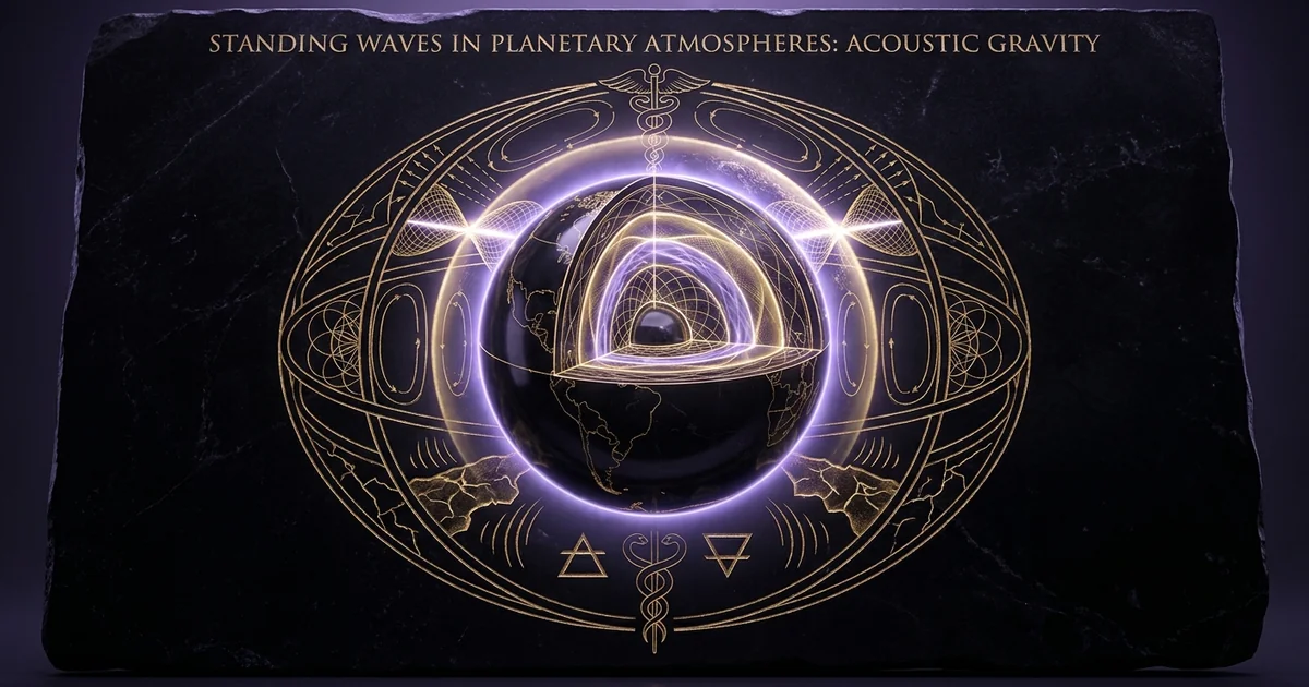
Standing Waves in Planetary Atmospheres: Acoustic Gravity
Executive Summary & Theoretical Thesis
The Planetary Atmosphere as a Stratified Resonator
A planetary atmosphere is not a quiescent, semi-infinite gas volume dissipating mechanical energy through isotropic radiative diffusion. Instead, it constitutes a geometrically bounded, continuously forced, stratified fluid resonant cavity. The vertical structure of the terrestrial atmosphere is defined by an exponential decay in ambient density $\rho_0(z) = \rho_0(0)\exp(-z/H)$, governed by the local scale height $H = k_B T / (m g)$, where $k_B$ is the Boltzmann constant, $T$ is absolute temperature, $m$ is mean molecular mass, and $g$ is the local gravitational acceleration.
This steep density gradient, paired with the non-monotonic vertical temperature profile dictated by radiative equilibrium in the mesosphere, stratosphere, and thermosphere, imposes rigorous mathematical boundary conditions upon acoustic propagation. Compressional mechanical waves originating within the lower troposphere or at the planetary surface cannot propagate vertically without undergoing dispersive phase modification and reflection.
Rather than diffusing freely into the vacuum of space, long-period acoustic energy is channeled, refracted, and trapped. The interplay between fluid compressibility and gravitational restoring forces generates a discrete spectrum of standing-wave-modes. The atmosphere thus behaves as an acoustic-gravity waveguide, transforming stochastic mechanical energy into coherent, macro-scale atmospheric acoustic gravity waves standing oscillations earth that span the entire geosphere.
Acoustic-Gravity Boundary Dynamics and Eigenfrequency Discretization
The fundamental dynamics of this stratified resonator depend on two characteristic frequencies that divide propagating and evanescent wave regimes: the acoustic cutoff frequency $\omega_a$ and the Brunt-Väisälä frequency $\omega_b$. When a fluid parcel is displaced vertically, compressibility acts as the primary restoring force at high frequencies, yielding acoustic waves modified by gravity. At lower frequencies, buoyant restoring forces dominate, giving rise to internal gravity waves. Between these two dynamic domains lies an evanescent passband where purely vertical propagation is prohibited, turning the atmospheric column into a reflective, phase-shifting boundary.
Because the planetary surface acts as an acoustically rigid boundary condition where the vertical perturbation velocity $w$ must vanish ($w(z=0) = 0$), and the upper atmospheric layers feature steep kinematic viscosity increases and thermal inversions that induce downward reflection, the atmosphere operates under discrete Sturm-Liouville boundary conditions. These boundaries discretize the continuous spectrum of mechanical perturbations into stable eigenmodes.
These planetary resonant acoustic modes exhibit both horizontal and vertical standing patterns. Along the horizontal axis, the continuous spherical shell requires periodic boundary conditions governed by Legendre polynomials, while vertical trapping between the planetary surface and the mesopause produces standing vertical nodes. Consequently, the atmospheric fluid column functions as an energetic filter that actively selects, amplifies, and sustains discrete vibrational frequencies from broadband mechanical excitation.
Coupling Mechanisms Across the Geosphere-Ionosphere Continuum
The formation of atmospheric acoustic gravity waves standing oscillations earth establishes a direct mechanical and electrodynamic conduit across traditionally compartmentalized planetary spheres. At the lower interface, the atmosphere couples to the lithosphere and hydrosphere. Microseismic noise generated by non-linear ocean wave interactions (the planetary “hum”) and tectonic displacements injects continuous, low-amplitude infrasound into the atmospheric waveguide.
As these acoustic waves propagate upward into regions of vanishing density, the conservation of vertical kinetic energy flux requires that the wave perturbation velocity increases exponentially with altitude:
$$u(z) \propto \rho_0(z)^{-1/2}$$
By the time these wavefronts reach the ionospheric E- and F-regions (90 to 350 km altitude), microscopic surface displacements on the order of nanometers to micrometers manifest as macroscopic neutral-gas velocity oscillations of tens to hundreds of meters per second.
Within the weakly ionized plasma of the ionosphere, these massive neutral-particle displacements drive charge separation via differential neutral-ion collision frequencies, directly modulating the ionospheric-dynamo. This acousto-electrodynamic coupling demonstrates that terrestrial standing acoustic modes are not mere barometric curiosities; they are foundational drivers of global ionospheric plasma variations, connecting the physical kinetics of the solid Earth directly to space-weather processes.
In a stratified, non-isothermal shear flow, the vertical structure of acoustic-gravity perturbations is formalized via the Taylor-Goldstein equation. Under an isothermal approximation with no background shear, the acoustic cutoff frequency $\omega_a$ and the Brunt-Väisälä (buoyancy) frequency $\omega_b$ are expressed as:
$$\omega_a = \frac{c_s}{2H} = \frac{\gamma g}{2 c_s}$$
$$\omega_b = \sqrt{\frac{g}{T}\left(\frac{dT}{dz} + \Gamma_d\right)} \xrightarrow{\text{isothermal}} \sqrt{\frac{(\gamma - 1)g^2}{c_s^2}} = \frac{g}{c_s}\sqrt{\gamma - 1}$$
where $c_s = \sqrt{\gamma R T}$ is the adiabatic speed of sound, $\gamma$ is the ratio of specific heats ($C_p/C_v \approx 1.4$ for diatomic air), and $\Gamma_d = g/C_p$ is the dry adiabatic lapse rate. For the standard terrestrial troposphere, nominal values are $\omega_a \approx 3.3 \text{ mHz}$ (period $\tau_a \approx 300 \text{ s}$) and $\omega_b \approx 2.9 \text{ mHz}$ (period $\tau_b \approx 330 \text{ s}$). Waves with frequencies $\omega > \omega_a$ reside in the acoustic branch, waves with $\omega < \omega_b$ occupy the internal gravity branch, and the interval $\omega_b < \omega < \omega_a$ constitutes an evanescent zone where waves decay exponentially with altitude unless sustained as boundary modes (e.g., Lamb waves).
Historical Lineage & Experimental Precedents
Classical Foundations: From Laplace’s Tidal Equations to Lamb Waves
The mathematical investigation of atmospheric fluid oscillations began with Pierre-Simon Laplace in his Mécanique Céleste (1799), wherein he formulated the Laplace Tidal Equations. Laplace modeled the atmosphere as a thin, barotropic fluid layer on a rotating sphere, attempting to quantify oceanic and atmospheric response to lunisolar gravitational potential.
While Laplace’s work treated oscillations as predominantly horizontal, hydrostatic phenomena, it established the framework for planetary-scale dynamic wave mechanics. A critical advancement occurred in 1910, when Sir Horace Lamb published his foundational treatise on the propagation of compression waves in a gravitationally stratified atmosphere.
Lamb demonstrated the existence of a unique, non-dispersive boundary wave—subsequently termed the lamb-waves—that propagates purely horizontally within an atmosphere bounded below by a solid plane. The Lamb wave is non-dispersive, possessing a horizontal phase velocity equal to the adiabatic speed of sound ($v_{ph} = c_s$). Its perturbation energy remains trapped near the surface, decaying exponentially with altitude according to:
$$p’(z) = p’(0)\exp\left(-\frac{\gamma g z}{c_s^2}\right)$$
Empirical verification of Lamb’s theoretical boundary waves arrived via the catastrophic cataclysm of the 1883 Krakatoa eruption. The barometric shockwaves generated by the volcanic collapse traversed the globe multiple times, recorded by mercury barographs worldwide as recurring, coherent pressure fluctuations with a period of roughly 36 to 40 hours per planetary circumnavigation. The Krakatoa pressure pulse confirmed that the planetary atmosphere acts as a low-loss spherical acoustic waveguide capable of sustaining coherent global waveforms across tens of thousands of kilometers.
The Mid-Century Infrasound Paradigm: Hines’ Ionospheric Gravity Waves
Throughout the early 20th century, observational upper-atmospheric physics encountered anomalous perturbations in meteor trail drifts and high-frequency radio soundings of the ionosphere. These high-altitude traveling ionospheric disturbances (TIDs) exhibited horizontal phase speeds of hundreds of meters per second and wavelengths spanning hundreds of kilometers, exceeding the velocity scales attributable to conventional tropospheric meteorology.
In a seminal 1960 paper, Colin O. Hines unified these disparate observations into a comprehensive hydrodynamical model of internal atmospheric gravity waves. Hines demonstrated that the upper atmosphere is systematically perturbed by waves generated in the lower atmosphere that propagate obliquely upward. Crucially, Hines formalized the vertical growth profile dictated by conservation of energy.
Because atmospheric density decreases by roughly nine orders of magnitude between sea level and the ionospheric F2-peak, any unattenuated upward-propagating acoustic-gravity wave must undergo a compensatory exponential amplitude increase. Hines proved that minor tropospheric pressure variances (fractions of a Pascal) inevitably manifest at 200 km altitude as massive wind oscillations (exceeding $50 \text{ m/s}$) and significant temperature fluctuations. This paradigm shifted upper-atmospheric mechanics from an isolated, solar-driven plasma regime to an integrated acousto-fluidic continuum coupled directly to lower-boundary mechanical forcing.
The theoretical transition from acoustic compression modes to buoyancy-dominated internal gravity waves is traced through two seminal primary texts:
-
Lamb, H. (1910). On Atmospheric Oscillations. Proceedings of the Royal Society of London. Series A, 84(573), 551–572. Lamb mathematically isolates the horizontal, non-dispersive acoustic boundary mode that preserves its vertical wave structure via gravitational equilibrium, establishing the surface boundary condition $w(0) = 0$ that underpins all subsequent planetary eigenmode models.
-
Hines, C. O. (1960). Internal Atmospheric Gravity Waves at Ionospheric Heights. Canadian Journal of Physics, 38(11), 1441–1481. Hines resolves the velocity amplification mechanics of upward-propagating infrasonic and gravity waves, deriving the horizontal and vertical wave dispersion relations in an isothermal stratified atmosphere, and directly correlating theoretical wave vectors to radar observations of ionized meteor trails.
Continuous Planetary Oscillation: The Discovery of Earth’s Acoustic Hum
For nearly a century, geophysicists assumed that the vibrational spectrum of the Earth was excited exclusively by discrete, transient dynamic events—namely earthquakes, volcanic eruptions, and artificial nuclear detonations. Between these catastrophic events, seismograms were presumed to measure only incoherent ambient noise generated by local meteorological and human interference.
This assumption was dismantled in the late 1990s through the deployment of ultra-broadband, low-noise seismometer networks (such as the Global Seismographic Network) and superconducting gravimeters. In 1998, researchers confirmed that the Earth undergoes continuous, unceasing planetary oscillations even during seismically quiescent periods.
Subsequent work by Nishida, Kobayashi, and Fukao (2000) revealed that this background hum is not confined to the lithosphere. By analyzing cross-correlations between superconducting gravimeter records and sensitive microbarometer networks, they proved that the Earth’s solid body and its atmospheric fluid envelope vibrate as an integrated, mechanically coupled dynamic system.
The background hum consists of discrete planetary resonant acoustic modes characterized by stable spectral peaks at millihertz frequencies, demonstrating that the entire planet is locked into permanent standing acoustic-gravity oscillations.
Mathematical Formalism & Physical Mechanics
Hydrodynamic Field Equations and the Stratified Dispersion Relation
The mechanics of atmospheric acoustic gravity waves standing oscillations earth derive from the fundamental equations of fluid dynamics: the Navier-Stokes equations, the equation of mass continuity, and the thermodynamic energy equation for an ideal gas. Neglecting viscous dissipation and Coriolis accelerations in the initial perturbation formulation, we consider an inviscid, non-rotating, gravitationally stratified fluid:
$$\frac{\partial \rho}{\partial t} + \nabla \cdot (\rho \mathbf{u}) = 0$$
$$\rho \left( \frac{\partial \mathbf{u}}{\partial t} + (\mathbf{u} \cdot \nabla)\mathbf{u} \right) = -\nabla p + \rho \mathbf{g}$$
$$\frac{\partial p}{\partial t} + \mathbf{u} \cdot \nabla p = c_s^2 \left( \frac{\partial \rho}{\partial t} + \mathbf{u} \cdot \nabla \rho \right)$$
where $\mathbf{u} = (u, v, w)$ is the velocity vector, $p$ is total pressure, $\rho$ is density, and $\mathbf{g} = -g \hat{\mathbf{z}}$ is the acceleration of gravity directed downward along the vertical coordinate $z$.
We apply Eulerian perturbation theory, decomposing each thermodynamic field into an unperturbed, hydrostatically balanced background state (denoted by subscript 0) and an infinitesimally small perturbation (denoted by prime):
$$p(\mathbf{r}, t) = p_0(z) + p’(\mathbf{r}, t)$$
$$\rho(\mathbf{r}, t) = \rho_0(z) + \rho’(\mathbf{r}, t)$$
$$\mathbf{u}(\mathbf{r}, t) = \mathbf{0} + \mathbf{u}'(\mathbf{r}, t)$$
The unperturbed state satisfies the hydrostatic equation:
$$\frac{dp_0}{dz} = -\rho_0(z) g$$
Linearizing the governing equations by discarding terms quadratic in the perturbations yields:
$$\frac{\partial \rho’}{\partial t} + w’ \frac{d\rho_0}{dz} + \rho_0 \nabla \cdot \mathbf{u}’ = 0$$
$$\rho_0 \frac{\partial \mathbf{u}‘}{\partial t} = -\nabla p’ + \rho’ \mathbf{g}$$
$$\frac{\partial p’}{\partial t} + w’ \frac{dp_0}{dz} = c_s^2 \left( \frac{\partial \rho’}{\partial t} + w’ \frac{d\rho_0}{dz} \right)$$
Assuming an isothermal background atmosphere wherein scale height $H = c_s^2 / (\gamma g)$ is constant, we apply a Fourier transform across space and time. Because the background state varies along the vertical axis $z$, perturbations do not take the form of standard planar waves. To eliminate the background density gradient from the differential equations, we execute the transformation:
$$\tilde{\mathbf{u}}(\mathbf{r}, t) = \sqrt{\rho_0(z)} \mathbf{u}'(\mathbf{r}, t) = \mathbf{U} \exp\left[ i(k_x x + k_y y + k_z z - \omega t) \right]$$
$$\tilde{p}(\mathbf{r}, t) = \frac{p’(\mathbf{r}, t)}{\sqrt{\rho_0(z)}} = P \exp\left[ i(k_x x + k_y y + k_z z - \omega t) \right]$$
where $k_h = \sqrt{k_x^2 + k_y^2}$ represents the horizontal wavenumber, $k_z$ is the vertical wavenumber, and $\omega$ is the angular frequency. Substituting these transformed variables into the linearized system produces the fundamental acoustic-gravity dispersion relation.
Following Sir James Lighthill’s classical formulation in Waves in Fluids (1978, Cambridge University Press), the dispersion relation governing waves in an isothermal, gravitationally stratified gas is:
$$\omega^4 - \omega^2 c_s^2 \left( k_h^2 + k_z^2 + \frac{1}{4H^2} \right) + (\gamma - 1) g^2 k_h^2 = 0$$
Expressing this relation in terms of the acoustic cutoff frequency $\omega_a = c_s / (2H)$ and the Brunt-Väisälä frequency $\omega_b = \frac{g}{c_s}\sqrt{\gamma - 1}$, the equation assumes the standard canonical form:
$$\omega^4 - \omega^2 c_s^2 \left( k_h^2 + k_z^2 \right) - \omega^2 \omega_a^2 + \omega_b^2 c_s^2 k_h^2 = 0$$
Rearranging for the vertical wavenumber $k_z^2$:
$$k_z^2 = \frac{\omega^2 - \omega_a^2}{c_s^2} - k_h^2 \left( 1 - \frac{\omega_b^2}{\omega^2} \right)$$
This dispersion equation defines whether an atmospheric perturbation exhibits oscillatory vertical propagation ($k_z^2 > 0$) or spatial evanescence ($k_z^2 < 0$).
Wave Vector Decomposition: Vertical Wavenumbers and Evanescent Regimes
The behavior of the vertical wavenumber $k_z$ dictates the morphological structure of the wavefield across the planetary vertical column:
-
Acoustic Branch ($\omega > \omega_a$): When the wave frequency exceeds the acoustic cutoff frequency, the term $(\omega^2 - \omega_a^2)$ is positive. For small horizontal wavenumbers, $k_z^2 > 0$, ensuring real values for $k_z$. These are modified acoustic modes. As $\omega \to \infty$, the equation asymptotically approaches the standard non-dispersive acoustic wave equation $\omega^2 = c_s^2 (k_h^2 + k_z^2)$. Compression and fluid inertia dominate; gravitational buoyancy acts as a minor dispersive perturbation.
-
Internal Gravity Branch ($\omega < \omega_b$): When the wave frequency falls below the Brunt-Väisälä frequency, $\omega^2 < \omega_b^2$, the factor $(1 - \omega_b^2/\omega^2)$ becomes negative. This negative sign reverses the balance, allowing $k_z^2 > 0$ for sufficiently large horizontal wavenumbers $k_h$. In this regime, the fluid moves almost along constant-density surfaces, tilted at an angle $\theta$ to the horizontal such that $\omega = \omega_b \cos\theta$. Restoring forces are entirely buoyant, arising from vertical parcel displacement within the stable density gradient.
-
Evanescent Bandgap ($\omega_b < \omega < \omega_a$): Within this intermediate frequency window, both terms work in tandem to drive $k_z^2 < 0$. The vertical wavenumber becomes purely imaginary:
$$k_z = i \kappa_z \quad \text{where} \quad \kappa_z = \sqrt{k_h^2 \left(1 - \frac{\omega_b^2}{\omega^2}\right) - \frac{\omega^2 - \omega_a^2}{c_s^2}}$$
In this regime, mechanical perturbations cannot transfer phase or kinetic energy vertically through propagating wavefronts. Instead, perturbation amplitudes decay exponentially with altitude.
This evanescent bandgap is the exact physical mechanism responsible for the trapping of standing waves. Wave energy launched upward from the troposphere within this frequency band is reflected by the stratified atmospheric column, turning the lower atmosphere into a high-Q acoustic resonator. The sole exception is the boundary-confined Lamb mode, which satisfies the condition $k_z^2 = 0$ along with a zero vertical velocity boundary condition across all heights.
Frequency (ω)
     ^
     |      ACOUSTIC BRANCH (Propagating: kz² > 0)
ω_a -+--------------------------------------------------- [Acoustic Cutoff]
     |      EVANESCENT BANDGAP (Reflective: kz² < 0)
ω_b -+--------------------------------------------------- [Brunt-Väisälä Frequency]
     |      INTERNAL GRAVITY BRANCH (Propagating: kz² > 0)
     +---------------------------------------------------> Horizontal Wavenumber (k_h)
Nonlinear Wave Steepening and Dissipation in the Thermosphere
For freely propagating waves that penetrate the evanescent barrier or reside outside its spectral limits, the conservation of energy flux dictates vertical amplification. In the absence of viscous dissipation, the vertical component of the wave energy flux vector $\mathbf{F}_g = \langle p’ \mathbf{u}’ \rangle$ must remain invariant with respect to altitude:
$$\frac{d}{dz} \langle p’(z) w’(z) \rangle = 0$$
Because the acoustic impedance of the medium scales with the background fluid density $\rho_0(z)$, the perturbation velocity $\mathbf{u}'(z)$ must scale inversely with $\sqrt{\rho_0(z)}$:
$$\mathbf{u}‘(z) = \mathbf{u}’(0) \sqrt{\frac{\rho_0(0)}{\rho_0(z)}} = \mathbf{u}'(0) \exp\left(\frac{z}{2H}\right)$$
In the terrestrial atmosphere, the scale height $H$ averages approximately $7 \text{ km}$. Consequently, for every $14 \text{ km}$ of vertical ascent, the ambient density $\rho_0(z)$ decreases by a factor of $e^2 \approx 7.39$, forcing the velocity perturbation $\mathbf{u}'$ to grow by a factor of $e \approx 2.718$.
At an altitude of $140 \text{ km}$ (twenty scale heights), the amplification factor reaches $\exp(10) \approx 22,026$. A seismic displacement or ocean wave convergence imparting a miniscule infrasonic perturbation of $1 \text{ mm/s}$ at sea level produces a velocity perturbation exceeding $22 \text{ m/s}$ in the thermosphere.
Altitude (z)
   ^
   |        Thermosphere (150 km)   --> Velocity u' amplified ~10^4 to 10^5
   |                                    Non-linear steepening, shock formation,
   |                                    viscous & radiative damping dominant.
   |
   |        Mesosphere (80 km)      --> Reflection at mesopause cold trap
   |
   |        Stratosphere (50 km)    --> Refraction via stratopause thermal maximum
   |
   |        Troposphere (0-12 km)   --> Surface boundary w(0)=0; microseismic forcing
  ---+--------------------------------------------------------------------------------> Perturbation Velocity u'
As perturbation velocities approach the local acoustic speed ($u’/c_s \sim \mathcal{O}(0.1 - 1.0)$), the linear assumption fails. Nonlinear terms $(\mathbf{u}’ \cdot \nabla)\mathbf{u}'$ in the Navier-Stokes equations produce progressive wave steepening: the compressional wave crests travel faster than the rarefaction troughs, transforming smooth sinusoidal waves into discontinuous acoustic shocks.
Concurrently, the molecular kinematic viscosity $\nu = \mu / \rho_0(z)$ increases exponentially with altitude. At thermospheric heights, viscous diffusion and thermal conduction attenuate these steepened waveforms, converting coherent standing-wave kinetic energy directly into localized thermal energy. This continuous dissipation process forms a major non-solar thermal input for the terrestrial upper atmosphere.
Empirical Evidence & Observational Data
Global Infrasound Monitoring Network (IMS) Array Telemetry
The theoretical framework of global atmospheric oscillations is verified by continuous data from the International Monitoring System (IMS) infrasound network, operated under the auspices of the Comprehensive Nuclear-Test-Ban Treaty Organization (CTBTO). The IMS network comprises roughly 60 operational infrasound stations distributed globally, each utilizing multi-channel arrays of spatial microbarometer sensors equipped with noise-reduction pipe manifolds. These microbarometers routinely resolve atmospheric pressure fluctuations across the $0.001 \text{ Hz}$ to $20 \text{ Hz}$ passband with sub-millipascal resolution.
Array telemetry consistently detects continuous, coherent infrasonic oscillations known as microbaroms. Arising from standing surface waves generated by counter-propagating ocean swell systems, microbaroms peak sharply within the spectral range of $0.1 \text{ Hz}$ to $0.5 \text{ Hz}$ (predominantly near $0.2 \text{ Hz}$). Cross-correlation of multi-array data demonstrates that these signals do not attenuate locally. Instead, they establish coherent global standing-wave interference fields that span entire ocean basins and continental interiors, utilizing the stratospheric-tropospheric wave guide to propagate across planetary distances.
       Tropospheric / Stratospheric Duct
  Z ^               Stratopause (High T, High c_s)
    |              /-------------------------------\   <- Downward Refraction
    |             /                                 \
    |  Source    /                                   \
    |    *======/                                     \======* Receiver (IMS Array)
  --+-----------------------------------------------------------> X
    0            Earth's Surface (Acoustic Rigid Boundary)
Beyond the microbarom spectrum, ultra-long-period microbarometric records reveal pervasive low-frequency background oscillations spanning the millihertz regime ($1 \text{ mHz} - 10 \text{ mHz}$). These signals match the fundamental eigenmodes of planetary atmospheric acoustic gravity waves standing oscillations earth, verifying that the atmospheric volume vibrates continuously in synchronized phase coherence with global geodynamic processes.
Doppler Ionosonde and Total Electron Content (TEC) Perturbations
Direct observation of the ionospheric manifestation of these standing modes is achieved through dual-frequency Global Navigation Satellite System (GNSS) receivers and vertical-incidence high-frequency (HF) Doppler sounding networks. GNSS signals traversing the ionospheric plasma experience a phase advance and group delay directly proportional to the line-of-sight integrated free electron density, known as the Total Electron Content (TEC):
$$\text{TEC} = \int_{s_{\text{rx}}}^{s_{\text{tx}}} N_e(s) , ds$$
where $N_e$ is the electron number density. High-rate GNSS telemetry networks (sampling at $\ge 1 \text{ Hz}$) systematically process carrier-phase observations to extract differential TEC perturbations ($\delta \text{TEC}$).
Following seismic rupture, volcanic detonation, or continuous microseismic forcing, $\delta \text{TEC}$ data display coherent, concentric, and standing traveling ionospheric disturbances (TIDs). These perturbations exhibit period bands identical to ground-level infrasonic modes ($100 \text{ s}$ to $600 \text{ s}$).
Continuous Doppler sounding arrays—which transmit stable HF carrier waves reflected off discrete ionospheric plasma layers back to ground receivers—demonstrate that the reflecting plasma mirror oscillates vertically with velocity amplitudes of $10 \text{ m/s}$ to $100 \text{ m/s}$. The detected phase velocities match the speed of acoustic-gravity wave propagation within the neutral thermosphere, proving that upward-propagating infrasound modulates the plasma geometry via neutral-ion drag.
Seismo-Acoustic Bimodal Resonances at 3.7 mHz and 4.4 mHz
The most precise experimental proof of continuous acoustic coupling between the solid Earth and its atmosphere emerged from cross-spectral analyses of superconducting gravimeters, broadband seismometers, and microbarographs. Nishida, Kobayashi, and Fukao (2000) demonstrated that the Earth’s continuous seismic hum contains two prominent, persistent spectral doublets located precisely at $3.7 \text{ mHz}$ ($\tau \approx 270 \text{ s}$) and $4.4 \text{ mHz}$ ($\tau \approx 227 \text{ s}$).
The physical mechanics governing atmospheric standing modes split across the evanescent bandgap, displaying opposing dynamic behaviors:
Acoustic Mode Resonance ($f > 3.3\text{ mHz}$)
- Restoring Force: Compressive atmospheric elasticity (fluid bulk modulus $K = \gamma p$).
- Particle Trajectory: Longitudinal, oscillating strictly parallel to the local wave propagation vector $\mathbf{k}$.
- Vertical Group Velocity: High vertical group velocity ($v_{gz} = \partial \omega / \partial k_z \sim c_s$).
- Dispersion Relation: $\omega^2 \approx c_s^2 (k_h^2 + k_z^2) + \omega_a^2$; phase and group velocity vectors are parallel ($\mathbf{v}_p \cdot \mathbf{v}_g > 0$).
- Primary Ionospheric Perturbation: Directly compresses the neutral gas and plasma, driving vertical oscillations observed as high-frequency Doppler ionosonde shifts and rapid $\delta\text{TEC}$ oscillations.
Internal Gravity Mode Resonance ($f < 3.0\text{ mHz}$)
- Restoring Force: Gravitational buoyancy acting on displaced stratified density parcels.
- Particle Trajectory: Highly elliptical to transverse, oriented nearly perpendicular to the wave propagation vector $\mathbf{k}$.
- Vertical Group Velocity: Dispersive and slow vertical group velocity; rapid horizontal transport ($v_{gh} \gg v_{gz}$).
- Dispersion Relation: $\omega^2 \approx \frac{\omega_b^2 k_h^2}{k_h^2 + k_z^2}$; phase and group velocity vectors are perpendicular ($\mathbf{v}_p \cdot \mathbf{v}_g = 0$), with phase propagation oriented downward when energy propagates upward.
- Primary Ionospheric Perturbation: Generates long-wavelength, slow-moving Traveling Ionospheric Disturbances (TIDs) that redistribute electron layers horizontally over hundreds of kilometers.
These doublets do not align with the isolated elastic free-oscillation spheroidal modes of an airless solid Earth (${0}S{29}$ and ${0}S{37}$). Instead, numerical coupling models reveal that they represent vertical acoustic eigenmodes of the coupled lithosphere-atmosphere system. The $3.7 \text{ mHz}$ mode reflects a resonant acoustic standing wave trapped between the planetary surface and the lower thermospheric temperature inversion, while the $4.4 \text{ mHz}$ mode represents the second harmonic trapped within the atmospheric cavity.
The mechanical quality factor $Q$ of these coupled modes ranges from 30 to 100, indicating an exceptionally efficient resonant circuit. Continuous microseismic background noise excites the atmospheric column, while resonant standing atmospheric infrasound exerts a reciprocal pressure back onto the crust, demonstrating bi-directional mechanical feedback.
Structural Architecture: Lithosphere-Atmosphere-Ionosphere Dynamic Coupling
Acousto-Electrodynamic Transduction at the E-Region Dynamo
The mechanical energy carried by vertically propagating standing infrasound transitions into electromagnetic energy within the lower ionosphere via the E-region dynamo (altitudes between $90 \text{ km}$ and $150 \text{ km}$). In this transition region, the neutral atmospheric density is low enough to permit free path lengths for ions, but high enough that the neutral-ion collision frequency $\nu_{in}$ remains substantially higher than the ion gyrofrequency $\Omega_i$:
$$\nu_{in} \gg \Omega_i = \frac{e B_0}{m_i}$$
where $e$ is elementary charge, $B_0$ is the geomagnetic field intensity, and $m_i$ is the mean ion mass.
Conversely, because the electron mass $m_e$ is negligible compared to the ion mass, the electron gyrofrequency $\Omega_e$ dwarfs the electron-neutral collision frequency $\nu_{en}$:
$$\Omega_e \gg \nu_{en}$$
Consequently, upward-propagating acoustic-gravity waves displace neutral gas molecules, which drag ions across the ambient geomagnetic field lines via dense collisional friction. The electrons, however, remain trapped by the Lorentz force, gyrating tightly around the geomagnetic field lines and unable to move across them along with the neutral flow. This differential motion between collisionally driven ions and magnetically confined electrons produces an acousto-electric current:
$$\mathbf{J}_{\text{ind}} = \sigma_P \left( \mathbf{E} + \mathbf{u}‘_n \times \mathbf{B}_0 \right) + \sigma_H \frac{\mathbf{B}_0 \times \left( \mathbf{E} + \mathbf{u}’_n \times \mathbf{B}_0 \right)}{B_0}$$
where $\sigma_P$ is the Pedersen conductivity, $\sigma_H$ is the Hall conductivity, $\mathbf{E}$ is the ambient polarization electric field, and $\mathbf{u}'_n$ is the acoustic perturbation velocity of the neutral gas.
Because the neutral velocity field $\mathbf{u}'n$ is periodic and represents a standing acoustic mode, the induced electric current $\mathbf{J}{\text{ind}}$ and associated magnetic field fluctuations $\Delta \mathbf{B}$ oscillate at the exact modal frequencies of the atmospheric acoustic gravity waves standing oscillations earth. The atmosphere thus functions as an acousto-electrodynamic transducer, transforming planetary mechanical oscillations directly into electromagnetic field variations.
Planetary Cymatics: Nodal Surface Patterns of Standing Infrasound
Because the terrestrial atmosphere forms a continuous spherical shell bounded by the solid Earth, global standing acoustic-gravity waves must conform to planetary spherical harmonics. The spatial distribution of perturbation pressure $p’(\theta, \phi, z, t)$ is modeled by solving the Helmholtz wave equation in spherical coordinates $(r, \theta, \phi)$:
$$p’(r, \theta, \phi, t) = \sum_{l=0}^{\infty} \sum_{m=-l}^{l} R_{nl}® Y_l^m(\theta, \phi) \exp(-i \omega_{nl} t)$$
where $Y_l^m(\theta, \phi)$ are spherical harmonic functions of degree $l$ and order $m$, and $R_{nl}®$ describes the radial (vertical) eigenfunction for radial node index $n$.
The planetary surface consequently acts as a macro-scale cymatic plate. The horizontal components of these spherical harmonics define static lines of zero pressure perturbation (nodal lines) and regions of maximum compression and rarefaction (antinodes).
These macro-scale standing patterns, termed cymatic-modal-nodes, establish stationary planetary pressure topographies. The nodal and antinodal distributions dictate preferential geographic regions for the accumulation of atmospheric kinetic energy, organizing mesoscale convective cells and modulating long-wavelength cloud band patterns. Rather than being distributed stochastically, ambient atmospheric mechanical energy is spatially focused along geometric coordinates determined by the spherical acoustic eigenvalues of the planet.
Planetary Cymatic Eigenmode Distribution
                       Degree l=3, Order m=0 (Zonal)
                         North Pole
                         +---------+
                        /   + + +   \    <- Antinodal Cap (Max Compression)
                       |-------------|   <- Nodal Line (Zero Perturbation)
                       |    - - -    |   <- Antinodal Zone (Rarefaction)
                       |=============|   <- Equator (Nodal Line)
                       |    + + +    |   <- Antinodal Zone (Compression)
                       |-------------|   <- Nodal Line (Zero Perturbation)
                        \   - - -   /    <- Antinodal Cap (Max Rarefaction)
                         +---------+
                         South Pole</code></pre>
Thermospheric Trapping and the Terrestrial Acoustic Waveguide
The survival of discrete standing modes depends on the vertical temperature structure of the terrestrial atmosphere. The atmosphere does not exhibit a constant lapse rate; it features two pronounced temperature inversions:
- The stratopause (altitude $\sim 50 \text{ km}$), where ozone absorption of ultraviolet radiation drives local temperatures up to roughly $270 \text{ K}$.
- The thermosphere (base at $\sim 85 \text{ km}$), where extreme ultraviolet and X-ray absorption elevates temperatures past $1000 \text{ K}$.
Because the acoustic speed is proportional to the square root of temperature ($c_s(z) = \sqrt{\gamma R T(z)}$), these temperature inversions act as continuous acoustic refraction barriers. An acoustic-gravity wave launched upward from the troposphere encounters an increasing sound speed in the stratosphere. According to Snell’s law of acoustic refraction:
$$\frac{\sin\theta(z)}{c_s(z)} = \text{constant}$$
where $\theta(z)$ is the angle of the wave vector relative to the vertical. As $c_s(z)$ increases, the wave vector bends away from the vertical until it reaches a critical turning point where $\sin\theta = 1$, refracting the wave energy back toward the solid surface.
Vertical Sound Speed Profile and Wave Trapping
 Altitude (z)
   ^
   |     \                   Thermosphere (T > 1000 K) -> High c_s: Upward Escape / Damping
   |      \
   |-------+                 Mesopause Cold Trap (T ~ 180 K) -> Lowest c_s
   |      /
   |     /                   Stratopause (T ~ 270 K) -> High c_s: Total Internal Reflection
   |    /
   |   /                     Troposphere / Ground -> Rigid Boundary w(0)=0
  -+--+--------------------> Sound Speed c_s(z)
     c_min                  c_max
The region between the planetary boundary layer and the mesopause cold trap (altitude $\sim 85 \text{ km}$, where temperatures drop to $\sim 180 \text{ K}$) forms an acoustic waveguide known as the thermospheric/mesospheric resonant cavity. Waves trapped within this cavity undergo continuous internal reflection between the ground and the upper refractive thermal barriers.
This acoustic ducting prevents infrasonic energy from dissipating directly into the exosphere, generating high-amplitude standing modes whose vertical Q-factors permit persistent structural resonance across planetary geodetic scales.
Metaphysical Implications & Unified Synthesis
The Planet as an Acoustic Instrument: Continuous Eigenmode Geometry
The demonstration that Earth’s atmosphere acts as a closed, stratified resonant cavity recontextualizes our understanding of planetary physics. Planetary bodies are not inert, passive lithospheric masses cushioned by formless atmospheric gas; they are integrated, self-organizing acoustic instruments. The physical dimensions of the planet—its surface gravity, atmospheric mass, mean molecular weight, and radius—function as intrinsic tuning parameters that define an invariant set of mechanical and electrodynamic eigenvalues.
This continuous acoustic oscillation removes the divide between “static structure” and “dynamic process.” The global acoustic-gravity spectrum shows that terrestrial matter is trapped in a permanent vibrational state. The atmosphere hums at millihertz frequencies, producing standing pressure nodes and antinodes that span mountain ranges, ocean basins, and ionospheric plasma belts. The terrestrial sphere operates as a dynamic, coherent resonator whose mechanical, fluid, and electromagnetic behaviors are phase-locked through acoustic-gravity wave mechanics.
Coherence Between Terrestrial Geospheres and Ancient Harmonic Models
The discovery of these global standing oscillations provides a physical framework for classical natural philosophy and ancient harmonic cosmology. Historical concepts of the musica universalis—the “harmony of the spheres” formalized by Pythagoras, Plato in the Timaeus, and Johannes Kepler in his 1619 treatise Harmonices Mundi—posited that geometric order and proportional harmonia govern celestial architecture.
While historical science dismissed these models as mystical projection, modern geophysics demonstrates that planetary bodies possess an intrinsic harmonic architecture. The coupled solid Earth-atmosphere system oscillates with discrete, mathematically ordered eigenfrequencies governed directly by spherical geometry:
$$f_{nl} \propto \sqrt{\frac{l(l+1) g H}{4\pi^2 R_E^2}}$$
where $R_E$ is the radius of the Earth, and $l$ is the harmonic degree.
The discrete doublets at $3.7 \text{ mHz}$ and $4.4 \text{ mHz}$, along with the global electromagnetic modes of the schumann-resonance ($7.83 \text{ Hz}$, $14.3 \text{ Hz}$, etc.), establish an empirical realization of harmonic planetary organization. The Earth does not experience silent structural equilibrium. It produces a persistent spectrum of harmonic standing modes that couple its deepest lithospheric roots to the outer boundary of its ionospheric plasma sheath.
The empirical verification of the Earth’s non-catastrophic, continuous planetary oscillation was formalized in Science:
Nishida, K., Kobayashi, N., & Fukao, Y. (2000). Resonant Oscillations Between the Solid Earth and the Atmosphere. Science, 287(5461), 2244–2246.
Nishida et al. deployed cross-spectral analysis across global superconducting gravimeter arrays and seismic networks, isolating discrete background modes at $3.7\text{ mHz}$ and $4.4\text{ mHz}$ with mechanical coherence persisting indefinitely. Their derivations demonstrated that atmospheric acoustic-gravity standing modes couple with Rayleigh surface waves on the solid Earth, proving that planetary geometry directly determines a continuous, background mechanical hum without requiring seismic triggers.
Thermodynamic Dissipation and Geometrical Order in Planetary Systems
The existence of standing acoustic-gravity wave regimes alters how mechanical energy moves through the Earth system. Following the non-equilibrium thermodynamics of Ilya Prigogine, open systems driven far from thermodynamic equilibrium spontaneously generate ordered dissipative structures that maximize the efficiency of energy processing. The planetary atmosphere, driven by solar radiative flux and internal geothermal dissipation, utilizes standing acoustic-gravity modes as an organized mechanism for mechanical energy distribution.
Rather than allowing mechanical energy from ocean currents, orographic winds, and tectonic stresses to degrade directly into microscopic heat at the boundary layer, the stratified atmosphere channels this kinetic energy into coherent, macro-scale standing modes.
These modes transport coherent momentum and energy upward, driving secondary electrodynamic currents in the ionosphere and organizing upper-atmospheric plasma distribution before dissipating via viscous shock mechanics in the thermosphere. The atmosphere operates as an acoustic engine, transforming stochastic fluid turbulence into macroscopic geometric order and reinforcing the thermodynamic stability of the terrestrial geosphere.
Frequently Asked Questions
Mechanisms of Energy Retention in the Leaky Atmospheric Cavity
The Earth’s atmosphere lacks a rigid physical ceiling; its density decreases continuously toward the interplanetary exosphere. The maintenance of high-Q standing wave modes within such an open, “leaky” cavity depends on two primary trapping mechanisms: acoustic-gravity evanescence and steep refractive temperature gradients.
Within the evanescent frequency bandgap ($\omega_b < \omega < \omega_a$), the atmospheric medium cannot support real vertical phase propagation. Waves generated at the planetary surface within this spectrum encounter an imaginary vertical wavenumber ($k_z = i \kappa_z$). The fluid layer acts as an impedance mismatch barrier, reflecting the wave energy downward with a reflection coefficient approaching unity:
$$|R|^2 = \left| \frac{Z_{\text{upper}} - Z_{\text{lower}}}{Z_{\text{upper}} + Z_{\text{lower}}} \right|^2 \approx 1$$
Furthermore, the sharp temperature minimum at the mesopause cold trap (around $85 \text{ km}$) creates a pronounced sound speed discontinuity. Waves entering this zone experience total internal reflection if their incident angles exceed the critical angle dictated by Snell’s law.
While high-frequency wave packets can leak through the thermospheric ceiling and dissipate through molecular viscosity, the fundamental modal frequencies—particularly the $3.7 \text{ mHz}$ and $4.4 \text{ mHz}$ seismo-acoustic resonances—satisfy the spatial phase-matching conditions required to form destructive interference in the upward-leaking channel and constructive standing interference between the stratopause and the lithosphere. The cavity’s leakiness is thus restricted to narrow spectral leakage bands, preserving the standing modes indefinitely.
Infrasound Detection Limits and Distinguishing Modes from Transient Storms
Differentiating continuous planetary acoustic-gravity eigenmodes from transient infrasonic sources (such as severe convective supercells, volcanic explosions, bolide entries, or anthropogenic detonations) requires spatial cross-correlation and long-term array processing:
-
Spatial and Temporal Coherence: Transient events produce localized, expanding spherical or cylindrical wavefronts with finite, decaying duration and pronounced dispersion curves ($\partial^2 \omega / \partial k^2 \ne 0$). In contrast, planetary standing modes are temporally stationary and spatially coherent across global scales. Processing arrays apply frequency-wavenumber ($f$-$k$) analysis and beamforming algorithms across distributed networks (such as the IMS network), which isolates isotropic standing waves from directional, propagating transient wave packets.
-
Spectral Fingerprinting: Severe convective complexes and squall lines produce dynamic infrasound centered between $0.5 \text{ Hz}$ and $5 \text{ Hz}$, showing broad spectral variance that correlates directly with storm life cycles. Volcanic and bolide transients generate impulse signatures characterized by sharp, shock-like Lamb wave signatures followed by acoustic-gravity dispersion tails. Conversely, planetary acoustic-gravity modes manifest as invariant, ultra-narrow spectral doublets at millihertz frequencies ($3.7 \text{ mHz}$ and $4.4 \text{ mHz}$), maintaining phase stability across months and years of continuous observation regardless of localized tropospheric weather patterns.
The Quantitative Coupling Ratio Between Infrasound and Ionospheric Plasma
The mechanical-to-plasma energy transfer ratio between tropospheric infrasound and ionospheric plasma is non-linear and governed by the vertical atmospheric density gradient. At ground level, typical ambient continuous infrasonic pressure perturbations range from $1 \text{ mPa}$ to $100 \text{ mPa}$ ($\Delta p / p_0 \sim 10^{-8}$ to $10^{-5}$), generating negligible fractional displacement of the neutral gas.
As these waves propagate upward to the ionospheric F2-peak ($250 \text{ km}$ to $350 \text{ km}$), the background neutral density drops by roughly nine orders of magnitude:
$$\frac{\rho_0(300\text{ km})}{\rho_0(0)} \approx 10^{-9}$$
Because kinetic energy flux density $\frac{1}{2}\rho_0 u’^2 c_s$ is conserved in the absence of severe damping, the perturbation velocity amplifies by a factor of $\sqrt{10^9} \approx 31,600$. A ground perturbation of $u’(0) = 1 \text{ mm/s}$ amplifies to a thermospheric velocity perturbation of $u’(300\text{ km}) \approx 31.6 \text{ m/s}$.
Within the weakly ionized plasma, the neutral gas transfers momentum to the electron and ion populations via Coulomb collisions. The quantitative coupling ratio—expressed as the fractional change in Total Electron Content relative to the driving surface pressure perturbation—scales as:
$$\frac{\delta\text{TEC}}{\text{TEC}_0} \approx \beta \left( \frac{u’_n}{c_s} \right) \sin I \cos\theta$$
where $\beta$ is a plasma compressibility factor ($\approx 0.5 - 1.2$), $I$ is the geomagnetic inclination angle, and $\theta$ is the angle between the neutral wave vector and the magnetic field lines.
Under resonant modal conditions, sub-Pascal surface microbarometric anomalies regularly produce macroscopic variations of $0.1$ to $2.0 \text{ TECU}$ ($1 \text{ TECU} = 10^{16} \text{ electrons/m}^2$), representing an ionospheric perturbation of $1%$ to $10%$ against background plasma density. This confirms that minute lithospheric and lower-atmospheric mechanical vibrations exert primary physical control over upper-atmospheric space plasma morphology. :::