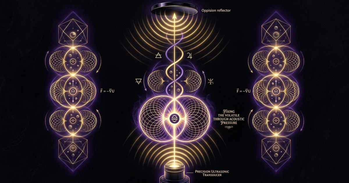
Single-Axis Acoustic Trapping: Standing Wave Force Wells
Executive Summary & Theoretical Thesis
Acoustic Radiation Force Topology in Uniaxial Cavities
Single-axis acoustic levitation relies on the non-linear mechanics of acoustic radiation pressure within an interferometric resonant cavity. When an emitter generates a coherent longitudinal ultrasonic wave that impinges upon an opposing boundary, the superposition of the incident and reflected waves establishes a stationary spatial distribution of pressure and velocity fields. In a classic single axis acoustic levitator standing wave ultrasonic reflector configuration, the primary mechanical translation of suspended matter is governed not by instantaneous oscillatory forces—which time-average to zero over an acoustic period $\tau = 2\pi/\omega$—but by second-order, non-zero time-averaged momentum transfers from the acoustic field to the particulate boundary.
The spatial topology of this standing wave field is defined by alternating velocity antinodes (pressure nodes) and velocity nodes (pressure antinodes) spaced at regular half-wavelength ($\lambda/2$) intervals along the propagation axis $z$. For a particle whose characteristic radius $R$ satisfies the Rayleigh scattering limit ($R \ll \lambda$), the acoustic radiation force vector $\mathbf{F}^{\text{rad}}$ emerges as the negative gradient of an acoustic potential field. In a purely one-dimensional ideal standing wave, the spatial distribution of this field concentrates matter into discrete planar levitation zones.
However, macroscopic physical trapping demands three-dimensional confinement. While axial positioning is achieved through the counteraction of gravitational acceleration by the primary axial acoustic radiation pressure gradient, lateral retention necessitates a non-zero radial acoustic restoring force. This radial force arises from cross-axis velocity gradients, transducer edge-diffraction effects, and wavefront curvature imparted by boundary geometries, establishing closed potential wells in three-dimensional space.
Pressure Distribution in Standing Wave Cavity
    Transducer
    [========]  z = 0 (Velocity Antinode / Pressure Node or Antinode depending on phase)
        |
        :       p(z) = 2*p_0 * cos(k*z)
        |
      ( o )     z = lambda/4 (Pressure Node: Stable Equilibrium for Dense Particles)
        |
        :       Maximum Velocity Gradient / Zero Acoustic Pressure
        |
      =====     z = lambda/2 (Pressure Antinode: Dispersion Barrier)
        |
    [~~~~~~~~]  z = H = n*(lambda/2) (Concave Reflector Surface)
The Gor’kov Potential Landscape and Kinetic Equilibrium
The theoretical description of force distribution on small spherical inclusions within an inviscid fluid was formulated by L. P. Gor’kov in 1962, unifying earlier formulations by King (1934) and Yosioka and Kawasima (1955). Gor’kov demonstrated that the time-averaged acoustic radiation force acting on a Rayleigh particle can be expressed as:
$$\mathbf{F}^{\text{rad}} = -\nabla U$$
where $U$ is the Gor’kov acoustic radiation potential. This scalar potential represents the net interaction of the particle’s volume with the local time-averaged acoustic kinetic energy density $\langle E_{\text{kin}} \rangle$ and acoustic potential (compressional) energy density $\langle E_{\text{pot}} \rangle$.
For a spherical body of radius $R$, density $\rho_p$, and compressional wave speed $c_p$ immersed in an ambient fluid medium of density $\rho_0$ and speed of sound $c_0$, the Gor’kov potential $U$ is defined as:
$$U = 2\pi R^3 \left[ \frac{\langle p_1^2 \rangle}{3 \rho_0 c_0^2} f_1 - \frac{\rho_0 \langle \mathbf{v}_1^2 \rangle}{2} f_2 \right]$$
Here, $\langle p_1^2 \rangle$ denotes the mean-square acoustic pressure fluctuation, $\langle \mathbf{v}_1^2 \rangle$ denotes the mean-square acoustic particle velocity vector, and the dimensionless acoustic contrast factors are formulated as:
$$f_1 = 1 - \frac{\kappa_p}{\kappa_0} = 1 - \frac{\rho_0 c_0^2}{\rho_p c_p^2}$$
$$f_2 = \frac{2(\rho_p - \rho_0)}{2\rho_p + \rho_0}$$
The parameter $\kappa_p = 1/(\rho_p c_p^2)$ is the isothermal compressibility of the particle, and $\kappa_0 = 1/(\rho_0 c_0^2)$ is that of the surrounding fluid. Dimensional verification demonstrates: $$[U] = [\text{Length}]^3 \cdot \left[ \frac{[\text{Pressure}]^2}{[\text{Density}][\text{Velocity}]^2} \right] = \text{m}^3 \cdot \left[ \frac{\text{N}^2 \cdot \text{m}^{-4}}{(\text{kg}\cdot\text{m}^{-3})(\text{m}^2\cdot\text{s}^{-2})} \right] = \text{N}\cdot\text{m} = \text{Joules}$$ The acoustic radiation force $\mathbf{F}^{\text{rad}} = -\nabla U$ yields dimensions of $\text{J}\cdot\text{m}^{-1} = \text{Newtons}$.
Equilibrium particulate trapping occurs at points where $\nabla U = 0$ alongside a positive definite Hessian matrix $\mathbf{H}_{ij} = \frac{\partial^2 U}{\partial x_i \partial x_j}$, ensuring a true local potential minimum. For the vast majority of solid particulate matter and liquid droplets suspended in gaseous media (such as ambient air, where $\rho_p \gg \rho_0$ and $\kappa_p \ll \kappa_0$), both contrast factors approach their upper limits: $f_1 \to 1$ and $f_2 \to 1$. Consequently, the composite acoustic contrast factor:
$$\Phi = \frac{f_1}{3} + \frac{f_2}{2}$$
remains strictly positive ($\Phi \approx 5/6$). Under these conditions, the Gor’kov potential is dominated by the pressure term, forcing particles to migrate away from regions of high pressure variance toward the velocity antinodes, which correspond to the pressure nodes of the standing wave field.
The balance of mechanical forces along the vertical axis defines the axial trapping stability. A trapped particle of mass $m = \frac{4}{3}\pi R^3 \rho_p$ experiences downward acceleration due to the gravitational field $\mathbf{g} = -g \hat{\mathbf{z}}$. Stable suspension is achieved when the vertical component of the radiation force matches and opposes gravity:
$$F_z^{\text{rad}}(z_{\text{eq}}) = m g$$
Because $F_z^{\text{rad}}$ varies sinusoidally along the $z$-axis with spatial periodicity $\lambda/2$, the particle does not reside precisely at the pressure node ($z = \lambda/4$) when subject to external acceleration. Instead, it settles at an offset equilibrium position $z_{\text{eq}} < \lambda/4$ where the local slope of the acoustic potential produces an upward restoring force equal to the gravitational load.
Concurrently, stability along the horizontal plane demands a restorative radial acoustic restoring force directed toward the central propagation axis ($r = 0$). In an idealized plane wave resonator, $\partial U / \partial r = 0$, meaning the radial restoring force vanishes, leading to instantaneous lateral ejection due to convective air currents or asymmetric acoustic scattering. Practical single-axis acoustic levitators overcome this limitation by tailoring the geometry of the acoustic cavity to generate lateral pressure gradients $\partial \langle p_1^2 \rangle / \partial r > 0$. This stabilizes the sample within three-dimensional energy force wells, linking the mechanical performance directly to the underlying wave geometry. For deeper insights into planar wave boundary interactions, see /sound-cymatics/chladni-plate-mathematics.
Historical Lineage & Experimental Precedents
Early Piezoelectric Resonators and Kundt Tube Ancestry
The historical trajectory of acoustic radiation force manipulation began with classical nineteenth-century acoustic investigations into stationary gas oscillations. August Kundt’s 1866 introduction of the dust-tube apparatus established the foundational visual paradigm for acoustic standing waves. By driving an enclosed cylindrical glass cavity with a frictionally excited metal rod, Kundt observed that lycopodium spores distributed throughout the lumen segregated into regular, periodic transverse striations. Although initially interpreted merely as a diagnostic technique for calculating the phase velocity of sound in gases, Kundt’s experiments represented the first macroscopic visualization of acoustic force wells structuring distributed matter.
Kundt, A. (1866). “Ueber eine neue Art Akustischer Staubfiguren und über die Anwendung derselben zur Bestimmung der Schallgeschwindigkeit in festen Körpern und Gasen.” Annalen der Physik und Chemie, 203(4), 497-523.
King, L. V. (1934). “On the acoustic radiation pressure on spheres.” Proceedings of the Royal Society of London. Series A, 147(861), 212-240.
The transition from passive boundary striations to active vertical levitation against gravity required high-frequency electromechanical actuation capable of generating significant acoustic energy densities. This transition accelerated following Paul Langevin’s development of quartz piezoelectric transducers for underwater echo-ranging during the First World War.
In 1933, Karl Bücks and H. Müller observed the levitation of alcohol droplets and particulate aerosols in a standing wave cavity powered by an x-cut quartz crystal operating in the megahertz regime. Bücks and Müller documented that small droplets positioned between the oscillating quartz face and an opposing boundary remained suspended against gravity. This definitively proved that acoustic radiation pressure could sustain steady-state momentum transfer to unconfined liquid volumes.
Historical Development Timeline of Acoustic Manipulation Mechanics:

1866: Kundt Dust Tube --------> 1933: Bücks & Müller --------> 1934: King Formulation
      Periodic particulate           Piezoelectric quartz           First analytical derivation
      striations in resonant         ultrasonic droplet             of radiation pressure on
      glass cylinders                trapping against gravity       rigid spherical bodies
                                                                               |
1962: Gor'kov Scalar Field <--- 1955: Yosioka & Kawasima <---------------------'
      Arbitrary sound fields;         Extension to compressible
      unification of potential        spheres in stationary
      gradient mechanics              fluid domains
Analytical Formulations: King, Yosioka-Kawasima, and Gor’kov
While experimental demonstrations confirmed that standing wave fields exert measurable mechanical forces, early mathematical models were limited by idealized hydrodynamic assumptions. The first rigorous mathematical treatment of radiation pressure was derived by Louis Vessot King in 1934. King examined the acoustic radiation pressure exerted by plane progressive and stationary waves on a rigid, incompressible sphere suspended in an inviscid fluid. By integrating the mean acoustic momentum flux across the oscillating sphere’s surface using spherical harmonic expansions, King demonstrated that the force is proportional to the acoustic energy density and scales directly with the volume of the sphere ($V \propto R^3$).
King’s model, however, was fundamentally constrained by the assumption of infinite particle rigidity ($\kappa_p \to 0$). In 1955, Keisuke Yosioka and Yukitaka Kawasima published an analytical framework that extended King’s formulation to compressible fluid and solid spheres. Their calculations accounted for the compressional waves scattered into the internal volume of the sphere, revealing that the direction of the acoustic radiation force depends directly on the relative compressibility contrast ($\kappa_p / \kappa_0$) and density contrast ($\rho_p / \rho_0$) between the particle and the host medium.
Lev Petrovich Gor’kov unified these mechanics in 1962. Recognizing that solving boundary value problems for individual particulate geometries in arbitrary wave configurations was computationally inefficient, Gor’kov reframed the radiation force problem through time-averaged thermodynamic stress tensors and potential theory. By introducing the scalar potential function $U$, Gor’kov reduced the complex computation of non-linear surface integral stresses to a straightforward calculation: evaluating the negative spatial gradient of an energy density field. This formulation remains the theoretical bedrock of modern acoustofluidics, particle sorting, and acoustic levitation design.
Transition from Micro-Particle Manipulation to Macroscopic Trapping
Throughout the latter half of the twentieth century, research shifted from analytical derivations toward physical systems engineering, driven largely by materials science requirements in microgravity environments. NASA and the European Space Agency (ESA) recognized that acoustic radiation pressure could enable containerless processing of molten high-purity semiconductors, refractory metals, and metastable glasses, eliminating the wall-induced heterogeneous nucleation inherent to traditional crucibles.
Ground-based experiments, however, faced the challenge of overcoming Earth’s 1-g gravitational acceleration. Suspending materials with densities exceeding $10^3\text{ kg/m}^3$ in ambient air ($\rho_0 \approx 1.2\text{ kg/m}^3$) demanded acoustic pressure amplitudes approaching $160\text{ to }170\text{ dB}$ SPL. At these intensities, non-linear harmonic distortion, acoustic streaming, and thermal dissipation become primary engineering constraints. Researchers developed specialized transducer horn assemblies (Langevin-type sandwich transducers) and high-reflectivity acoustic reflectors, transforming the simple single axis acoustic levitator standing wave ultrasonic reflector into a precision laboratory instrument. For an expanded analysis of multi-dimensional energy well generation, explore /sound-cymatics/acoustic-levitation-principles.
Mathematical Formalism & Physical Mechanics
Boundary Value Solutions of the Helmholtz Equation
The propagation and steady-state interference of longitudinal ultrasonic waves within an idealized one-dimensional acoustic cavity is governed by the classical linear wave equation for the acoustic velocity potential $\psi(\mathbf{r}, t)$:
$$\nabla^2 \psi - \frac{1}{c_0^2}\frac{\partial^2 \psi}{\partial t^2} = 0$$
Assuming time-harmonic excitation at angular frequency $\omega = 2\pi f$, the spatial dependency of the field is described by the Helmholtz equation:
$$\nabla^2 p_1 + k^2 p_1 = 0$$
where $p_1(\mathbf{r})$ is the complex acoustic pressure perturbation, $k = \omega/c_0 = 2\pi/\lambda$ is the acoustic wavenumber, and the physical acoustic pressure is given by $p(\mathbf{r}, t) = \text{Re}{p_1(\mathbf{r}) e^{-i\omega t}}$. The acoustic particle velocity field $\mathbf{v}_1$ is subsequently derived from Euler’s linearized momentum equation:
$$\rho_0 \frac{\partial \mathbf{v}_1}{\partial t} = -\nabla p_1 \quad \implies \quad \mathbf{v}_1 = \frac{1}{i \omega \rho_0} \nabla p_1$$
In a single-axis system aligned along the $z$-axis, we define the acoustic emitter boundary at $z = 0$ and the reflector surface at $z = H$. Modeling the emitter as an oscillating piston with normal velocity amplitude $v_0$ yields the inhomogeneous Neumann boundary condition:
$$\left. \frac{\partial p_1}{\partial z} \right|_{z=0} = -i \omega \rho_0 v_0$$
For a planar reflector with infinite acoustic impedance ($Z_{\text{reflector}} \gg Z_{\text{medium}}$), the fluid velocity normal to the boundary must vanish identically, imposing a homogeneous Neumann boundary condition:
$$\left. \frac{\partial p_1}{\partial z} \right|_{z=H} = 0$$
Solving the one-dimensional Helmholtz equation subject to these boundary parameters yields the complex pressure distribution within the resonant gap:
$$p_1(z) = -i \rho_0 c_0 v_0 \frac{\cos[k(H - z)]}{\sin(k H)}$$
The corresponding axial particle velocity profile evaluates to:
$$v_{1,z}(z) = v_0 \frac{\sin[k(H - z)]}{\sin(k H)}$$
These boundary value expressions demonstrate that the internal pressure and velocity fields diverge as $\sin(k H) \to 0$, which marks the mathematical condition for unbounded cavity resonance in the absence of viscous dissipation.
Transducer Reflector Distance Calibration and Cavity Resonance
The mechanical amplification of acoustic radiation pressure inside the levitator depends on transducer reflector distance calibration. Cavity resonance occurs when the acoustic path length accommodates an integer number of half-wavelengths:
$$H_n = n \frac{\lambda}{2} = n \frac{c_0}{2 f}, \quad n \in {1, 2, 3, \dots}$$
Under this resonant condition, constructive interference maximizes the acoustic energy density within the cavity. However, real-world acoustic cavities exhibit finite energy dissipation caused by bulk viscous damping, thermal conduction within oscillatory boundary layers, and acoustic radiation losses through open radial boundaries.
The quality factor $Q$ of the cavity quantifies this energy storage efficiency:
$$Q = \omega \frac{\mathcal{E}{\text{stored}}}{\mathcal{P}{\text{dissipated}}}$$
where $\mathcal{E}{\text{stored}}$ is the time-averaged acoustic energy stored within the cavity volume $V$, and $\mathcal{P}{\text{dissipated}}$ is the time-averaged rate of energy dissipation. With ambient air attenuation and boundary layer shearing, typical single-axis ultrasonic levitators operating at $f = 40\text{ kHz}$ ($\lambda \approx 8.65\text{ mm}$) achieve quality factors between $20 \le Q \le 150$.
When the separation distance $H$ deviates from resonance by an offset $\Delta H$, the standing wave ratio ($SWR$) degrades rapidly. The pressure amplitude inside the cavity scales as:
$$|p_{\text{max}}| \propto \frac{1}{\sqrt{\sin^2(k H) + \left(\frac{1}{Q}\right)^2 \cos^2(k H)}}$$
A misalignment $\Delta H$ as small as $\lambda/20$ can reduce the acoustic energy density by over $70%$, directly degrading the axial radiation force. Precise transducer reflector distance calibration using micrometer positioning stages or closed-loop piezo-actuation is essential to maintain the high-amplitude standing wave necessary to overcome gravitational loads.
Cavity Energy Response vs. Separation Distance
    |p_max|^2
      ^                              H_n = n * (lambda / 2)
      |                                     |
 1.0 -|                                    / \
      |                                   /   \     High Q-factor
 0.8 -|                                  /     \    Narrow Resonance Band
      |                                 /       \
 0.5 -| - - - - - - - - - - - - - - - -/---------\- - - FWHM ~ 1/Q
      |                               /           \
 0.2 -|                              /             \
      |_____________________________/_______________ \________________> Distance (H)
                                   H_n - dH        H_n + dH
Axial Trapping Stability vs. Radial Restoring Force Dynamics
The physical criteria governing particulate equilibrium are decoupled into two orthogonal coordinate domains: axial trapping stability along the primary propagation vector $\hat{\mathbf{z}}$, and the radial acoustic restoring force acting within the transverse plane $\mathbf{r}_\perp = (x, y)$.
Axial trapping stability is evaluated through the first and second spatial derivatives of the Gor’kov acoustic radiation potential along $z$. Substituting the 1D standing wave solutions for pressure and velocity into Gor’kov’s potential equation gives:
$$U(z) = \pi R^3 E_{\text{ac}} \left[ \frac{2}{3} f_1 \cos^2(kz) - f_2 \sin^2(kz) \right]$$
where $E_{\text{ac}} = \frac{p_0^2}{4 \rho_0 c_0^2}$ represents the characteristic acoustic energy density. Differentiating $U(z)$ with respect to $z$ yields the axial radiation force:
$$F_z^{\text{rad}}(z) = -\frac{\partial U}{\partial z} = \frac{4}{3} \pi R^3 k E_{\text{ac}} \left( f_1 + \frac{3}{2} f_2 \right) \sin(2kz) = 4\pi R^3 k E_{\text{ac}} \Phi \sin(2kz)$$
Equilibrium occurs where the net vertical force vanishes:
$$\sum F_z = F_z^{\text{rad}}(z) - m g = 0$$
Dynamic stability demands that the equilibrium point behave as a mechanical restoring spring:
$$\kappa_z = -\left. \frac{\partial F_z^{\text{rad}}}{\partial z} \right|{z{\text{eq}}} = \left. \frac{\partial^2 U}{\partial z^2} \right|{z{\text{eq}}} > 0$$
Evaluating this condition demonstrates that stable trapping can only occur within spatial windows where $\cos(2k z_{\text{eq}}) > 0$, bounding valid equilibrium positions to the lower half of each pressure nodal domain ($0 < z - z_{\text{node}} < \lambda/8$).
Vertical Force Equilibrium Vector Decomposition
+z ^
| F_rad(z) = 4*pi*R^3 * k * E_ac * Phi * sin(2kz)
| [Acoustic Radiation Force Vector]
|
.---[ O ]---. <--- Particle Mass Center
|
|
| F_g = m * g
| [Gravitational Force Vector]
-z v
Equilibrium Condition: F_rad(z_eq) - m*g = 0
Stability Requirement: d^2 U / dz^2 > 0 (Trap Stiffness kappa_z > 0)</code></pre>
Conversely, radial confinement cannot be sustained in a purely planar standing wave. If the acoustic field has no transverse dependence, $\partial U / \partial r = 0$, resulting in zero radial restoring force ($F_r^{\text{rad}} = 0$). Any lateral perturbation—such as ambient thermal convection, asymmetric boundary layer separation, or off-axis acoustic scattering—causes the particle to drift radially outward until it is ejected from the cavity.
To introduce a finite trap stiffness $\kappa_r = -\partial F_r / \partial r > 0$, the acoustic phase fronts must exhibit spatial curvature. This is typically achieved by substituting the planar reflector with a spherical concave reflector. The curved boundary shapes the reflected wave fronts, introducing transverse gradients in the acoustic kinetic and potential energy distributions:
$$\frac{\partial \langle p_1^2 \rangle}{\partial r} \neq 0, \quad \frac{\partial \langle \mathbf{v}_1^2 \rangle}{\partial r} \neq 0$$
These transverse gradients generate an inward-directed radial acoustic restoring force:
$$F_r^{\text{rad}}(r, z) \approx -\pi R^3 \left[ \frac{f_1}{3 \rho_0 c_0^2} \frac{\partial \langle p_1^2 \rangle}{\partial r} - \frac{\rho_0 f_2}{2} \frac{\partial \langle \mathbf{v}_1^2 \rangle}{\partial r} \right]$$
This centripetal force confines the particle to the central axis of the acoustic cavity. For complementary insights into standing wave resonance dynamics, consult /physics-electromagnetism/standing-wave-resonators.
Empirical Evidence & Observational Data
Laser Doppler Vibrometry and Schlieren Field Visualization
Empirical validation of the theoretical models governing single-axis standing wave traps requires high-precision optical diagnostics. The mechanical properties of the acoustic field are measured via two complementary techniques: Laser Doppler Vibrometry (LDV) to map the mechanical velocity of the boundary surfaces, and Schlieren photography or Mach-Zehnder interferometry to visualize the spatial acoustic pressure distribution in the fluid.
Schlieren Phase Optical Diagnostic Setup
[Collimated LED] —> [ Resonant Cavity ] —> [ De-collimating Lens ] —> [ Knife Edge ] —> [ High-Speed CMOS ]
|
±-> Density Variations: delta_rho(z,r)
±-> Refractive Index: delta_n proportional to delta_p
±-> Visualizes Standing Wave Nodes as Dark Striations
Schlieren diagnostics exploit the piezo-optic effect: local fluctuations in medium density induce proportional variations in the refractive index:
$$\Delta n(z, r, t) = \left( \frac{\partial n}{\partial \rho} \right)_T \Delta \rho(z, r, t) = \frac{n_0 - 1}{\rho_0 c_0^2} p_1(z, r, t)$$
By synchronizing high-speed imaging arrays with the transducer excitation frequency, researchers can map the acoustic standing wave nodes as high-contrast dark bands, directly verifying the axial node distribution predicted by the Helmholtz equation.
Simultaneously, scanning Laser Doppler Vibrometry is used to map the active face of the piezoelectric transducer. These measurements consistently reveal that transducers rarely behave as ideal planar pistons. Instead, transverse flexural modes generate spatial variations in surface velocity:
$$v_0® \neq \text{const}$$
These non-uniformities distort the near-field acoustic landscape, creating localized phase discrepancies. If uncorrected, this uneven velocity profile degrades cavity resonance, shifting the calculated force well geometries and introducing lateral instabilities.
Non-Linear Acoustic Streaming and Boundary Layer Instabilities
While the Gor’kov potential framework provides an accurate model of acoustic radiation forces in ideal inviscid fluids, real-world levitation in ambient air is complicated by viscous dissipation. This dissipation produces steady, time-averaged fluid circulations known as acoustic streaming.
Acoustic streaming originates from the Reynolds stress tensor inside the oscillatory viscous boundary layer (the Stokes layer) along the solid boundaries of the cavity. The characteristic thickness of this boundary layer is given by:
$$\delta_\nu = \sqrt{\frac{2\nu}{\omega}}$$
where $\nu = \mu/\rho_0$ is the kinematic viscosity of the medium. For a system operating at $f = 40\text{ kHz}$ in air ($\nu \approx 1.5 \times 10^{-5}\text{ m}^2/\text{s}$), the boundary layer thickness is small: $\delta_\nu \approx 10.9\ \mu\text{m}$.
                 Acoustic Streaming Flow Field Geometries
       Transducer Boundary
       =========================================================
       ~~~~~~~~ Schlichting Inner Streaming Layer (delta_nu) ~~~~  v_streaming ~ O(v_1^2 / c_0)
       ---------------------------------------------------------
          (   )        (   )        (   )        (   )
         (  ^  )      (  v  )      (  ^  )      (  v  )    Rayleigh Outer Recirculation
        (   |   )    (   |   )    (   |   )    (   |   )   Vortices in Cavity Bulk
         (  v  )      (  ^  )      (  v  )      (  ^  )
          (   )        (   )        (   )        (   )
       ---------------------------------------------------------
       =========================================================
       Reflector Surface
Within this thin Stokes layer, intense shearing generates high-vorticity inner streaming (Schlichting streaming). Friction between this inner layer and the adjacent fluid drives large-scale recirculation vortices across the bulk cavity (Rayleigh streaming).
These acoustic streaming vortices superimpose an active hydrodynamic drag force $\mathbf{F}^{\text{drag}} = 6\pi \mu R (\mathbf{u}{\text{stream}} - \mathbf{v}{\text{particle}})$ onto the primary radiation force field $\mathbf{F}^{\text{rad}}$. When the acoustic drive amplitude increases, the velocity of these streaming loops scales quadratically:
$$u_{\text{stream}} \propto \frac{v_0^2}{c_0}$$
If the acoustic velocity amplitude $v_0$ is driven too high, streaming drag can exceed the lateral acoustic restoring forces. This triggers boundary layer instabilities that manifest as sample orbital precession, rapid rotational spin, or lateral sample ejection from the acoustic force well.
Parametric Calibration for Dense and Liquid Specimen Levitation
Levitating dense solid materials (such as tungsten carbide, with $\rho_p \approx 15,600\text{ kg/m}^3$) or low-surface-tension liquid droplets requires fine control over the cavity geometry. When levitating liquid droplets, the acoustic radiation pressure must not only support the droplet’s weight but also avoid inducing catastrophic surface deformation.
The acoustic radiation pressure distribution over a droplet’s surface is non-uniform, exerting high compressional stress at the droplet’s poles and lower stress at its equator. This pressure differential deforms the spherical droplet into an oblate spheroid. The extent of this deformation is governed by the acoustic capillary number:
$$\text{Ca}_{\text{ac}} = \frac{p_0^2 R}{\gamma \rho_0 c_0^2}$$
where $\gamma$ is the interfacial surface tension. Empirical studies demonstrate that when $\text{Ca}{\text{ac}}$ exceeds a critical threshold ($\text{Ca}{\text{ac}} \ge 0.95$), the droplet develops a sharp, unstable equatorial edge. This instability triggers Rayleigh-Taylor and Kelvin-Helmholtz instabilities, ultimately causing the droplet to atomize into satellite micro-droplets.
Planar Ultrasonic Reflectors
- Axial Trap Stiffness ($\kappa_z$): Maximized under ideal alignment due to the uniform planar reflection wave front; delivers peak theoretical axial radiation force along the central axis.
- Radial Restoring Force ($\kappa_r$): Extremely weak ($\kappa_r \to 0$); relies entirely on natural transducer edge-diffraction effects, leaving samples highly vulnerable to lateral drift and air currents.
- Angular Misalignment Sensitivity: Highly sensitive; an axial tilt angle $\theta > 1.5^\circ$ degrades standing wave interference, collapsing the cavity quality factor $Q$.
- Acoustic Streaming Profile: Produces broad, symmetrical Rayleigh streaming cells that exert significant destabilizing cross-axis drag on levitated matter.
Concave Ultrasonic Reflectors
- Axial Trap Stiffness ($\kappa_z$): Slightly attenuated off-center relative to planar boundaries, but maintains high axial stability across the central focal zone.
- Radial Restoring Force ($\kappa_r$): Exceptionally strong; wave front curvature generates steep transverse acoustic energy density gradients, increasing radial trap stiffness by $35%\text{ to }50%$.
- Angular Misalignment Sensitivity: Robust against minor angular misalignment; the concave curvature self-focuses reflected wave energy back toward the primary cavity axis.
- Acoustic Streaming Profile: Compresses and localizes streaming vortices toward the peripheral margins of the cavity, protecting the central nodal core from destabilizing convective drag.
Metaphysical Implications & Unified Synthesis
Standing Waves as Geometric Morphogenetic Fields
Beyond its applications in material handling and fluid physics, the spatial architecture of standing wave force wells offers a physical model for the interaction between wave mechanics and structured matter. In classical morphogenesis, as posited by theorists from Hans Driesch to Rupert Sheldrake, biological structures are guided by spatial morphogenetic fields—non-material energy boundaries that direct the physical positioning and differentiation of cells. A standing wave acoustic cavity functions as an empirical, classical realization of this principle: an invisible, continuous scalar field creates discrete potential wells that force disorganized matter into ordered spatial geometries.
In a single axis acoustic levitator standing wave ultrasonic reflector configuration, continuous longitudinal wave inputs generate discrete particulate nodes. When matter is introduced into this volume, it naturally aggregates along structural nodes governed by the acoustic contrast factor.
The acoustic wave landscape does not physically pull or manipulate matter through direct contact; instead, it shapes the surrounding space into an array of energy potential wells. The suspended material simply follows passive thermodynamic gradients, settling at local potential minima. This phenomenon illustrates a foundational concept in field theory: the physical morphology of matter can be dictated by stationary energy distributions within a continuous carrier medium. For a mathematical analysis of these spatial patterns across higher-dimensional surfaces, see /sacred-geometry/cymatic-harmonics-platonic-solids.
Morphogenetic Spatial Field Correspondence:
Continuous Acoustic Scalar Field:  p_1(r, z) = P_0(r) * cos(kz) * e^(-iwt)
                           │
                           ▼
Nonlinear Gor'kov Potential Landscape:  U(r, z) = 2*pi*R^3 * [ (f_1/3)*<p^2> - (f_2/2)*<v^2> ]
                           │
                           ▼
Spatial Matter Organization:  F = -grad(U)  ===>  Matter Segregates into Discrete Nodal Bands
Macro-Cymatics and Archaeoacoustic Coherence
This structural organization scales directly with wavelength. The field of archaeoacoustics provides evidence that ancient cultures incorporated acoustic resonance into the architecture of megalithic chambers and ceremonial spaces. Excavations at sites such as the Hypogeum of Ħal Saflieni in Malta, Newgrange in Ireland, and the subterranean chambers of the Giza Plateau demonstrate that these megalithic stone enclosures function as acoustic cavities with high quality factors ($Q$).
Jahn, R. G., Devereux, P., Ibison, M., Cook, J. V., & Welch, G. J. (1996). “Acoustical Resonances of Assorted Ancient Structures.” Journal of the Acoustical Society of America, 99(2), 647-648.
Watson, A., & Keating, D. (1999). “Architecture and sound: an acoustic analysis of megalithic monuments in prehistoric Britain.” Antiquity, 73(280), 325-336.
These megalithic chambers consistently exhibit modal resonances in the infrasonic and lower audible acoustic spectrum, specifically between $95\text{ Hz}$ and $130\text{ Hz}$. At these frequencies, the acoustic wavelengths ($\lambda \approx 2.6\text{ to }3.6\text{ m}$) align with the physical dimensions of the stone enclosures. Continuous vocalization or percussive excitation within these spaces establishes standing waves analogous to those in an ultrasonic trapping cavity.
At these low frequencies, the acoustic radiation force is insufficient to levitate dense stone blocks against Earth’s gravitational acceleration: the radiation force scales inversely with acoustic wavelength ($F^{\text{rad}} \propto k \propto 1/\lambda$) and requires high energy densities ($E_{\text{ac}} \propto p_0^2$). However, these macro-cavities generate pronounced spatial variations in sound pressure and acoustic streaming velocity. These distributions focus auditory perception and particulate matter (such as smoke, aerosols, and dust) into stable nodal configurations. The geometric design of these ancient enclosures reflects an empirical understanding of wave interference, demonstrating how architectural boundaries can manipulate the acoustic energy landscape within an enclosed space.
Scalar Trapping: Acoustic Nodes as Universal Invariance Models
At a theoretical level, the mechanics of acoustic nodal trapping reflect universal invariance principles found throughout modern field theories. The mathematical framework describing the Gor’kov force well:
$$\mathbf{F} = -\nabla U(\mathbf{r})$$
is structurally isomorphic to the potential formulations used in optical tweezers, magnetostatic traps, and the confinement of cold neutral atoms within crossed laser beam lattices (optical lattices).
                      Universal Trapping Field Isomorphism

 Acoustic Cavity:   longitudinal sound waves  ==>  delta_U_gorkov ==>  Particulate Nodes
 Optical Lattice:   electromagnetic waves    ==>  delta_U_dipole ==>  Neutral Atom Array
 Quantum Field:     metric / gauge waves     ==>  delta_U_scalar ==>  Mass Localization
In all these systems, the interference of linear wave modes generates a non-linear, time-averaged spatial potential well capable of trapping mass. In an acoustic standing wave, the linear pressure field $p_1(\mathbf{r}, t)$ generates a second-order radiation stress tensor:
$$\langle \mathbf{\Pi}{ij} \rangle = \left( \frac{\langle p_1^2 \rangle}{2 \rho_0 c_0^2} - \frac{\rho_0 \langle \mathbf{v}1^2 \rangle}{2} \right) \delta{ij} - \rho_0 \langle v{1,i} v_{1,j} \rangle$$
The divergence of this tensor gives rise to the acoustic radiation force.
This transformation illustrates how linear wave superposition can create localized, non-linear energy wells that stably confine mass. Investigating the stability of single-axis acoustic levitators provides a accessible, tabletop model for studying localized physical confinement, offering valuable insights into how energy fields structure matter across different domains of physics.
Frequently Asked Questions
Acoustic Pressure Node versus Antinode Localization
Why do solid particles migrate to acoustic pressure nodes while gaseous bubbles in liquids concentrate at pressure antinodes?
Particulate migration within an acoustic standing wave is dictated entirely by the sign of the composite acoustic contrast factor:
$$\Phi(\kappa_p, \kappa_0, \rho_p, \rho_0) = \frac{1 - \frac{\kappa_p}{\kappa_0}}{3} + \frac{\rho_p - \rho_0}{2\rho_p + \rho_0}$$
This factor determines whether the local Gor’kov potential $U$ exhibits a local minimum at a pressure node or at a velocity node.
For dense, low-compressibility solids suspended in gases or liquids (e.g., a polystyrene sphere or mineral dust in air), the inclusion is both denser ($\rho_p \gg \rho_0$) and less compressible ($\kappa_p \ll \kappa_0$) than the host medium. In this regime, both terms evaluate to positive quantities, resulting in $\Phi > 0$. The Gor’kov potential is dominated by the dynamic pressure term $\langle p_1^2 \rangle$. Because the force vector satisfies $\mathbf{F} = -\nabla U$, the particle is driven toward points that minimize dynamic pressure fluctuations—the acoustic pressure nodes (velocity antinodes).
Particulate Phase Mechanics vs. Acoustic Node Phase:
  Dense / Incompressible Body (Phi > 0):
  Migration Vector ----> [ Pressure Node / Velocity Antinode ]

  Compressible / Low-Density Body (Phi < 0):
  Migration Vector ----> [ Pressure Antinode / Velocity Node ]
Conversely, when an inclusion is substantially more compressible than the surrounding medium—such as a gaseous bubble suspended in water ($\kappa_{\text{gas}} \gg \kappa_{\text{water}}$)—the compressibility ratio $\kappa_p / \kappa_0$ dominates the contrast equation, driving the monopole contrast factor negative ($f_1 \ll 0$). This yields a negative composite acoustic contrast factor ($\Phi < 0$).
Consequently, the signs in the potential energy formulation invert. The gaseous bubble minimizes its thermodynamic energy by migrating to regions that maximize the local acoustic pressure variance—the acoustic pressure antinodes (velocity nodes). This phenomenon, known as the inverted Bjerknes effect, demonstrates that the acoustic radiation potential does not operate as an absolute mechanical barrier; rather, it functions as a relative contrast field governed by the material properties of the inclusion and its host medium.
Impact of Reflector Geometry on Radial Restoring Force
How does a spherical concave reflector generate a radial acoustic restoring force without disrupting axial trapping stability?
A planar ultrasonic reflector produces an idealized boundary where reflected wave vectors remain strictly antiparallel to the incident wave fronts ($\mathbf{k}_{\text{reflected}} = -k \hat{\mathbf{z}}$). While this maximizes axial standing wave interference along the $z$-axis, it fails to generate the transverse energy gradients required to stabilize particles radially ($\partial U / \partial r = 0$).
Replacing the planar boundary with a spherical concave reflector of radius of curvature $R_c$ introduces a radially varying boundary height profile:
$$z_{\text{boundary}}® = H_0 + \left( R_c - \sqrt{R_c^2 - r^2} \right) \approx H_0 + \frac{r^2}{2 R_c}$$
This geometric curvature modifies the acoustic reflection boundary condition:
$$\hat{\mathbf{n}} \cdot \nabla p_1 = 0$$
where the surface normal unit vector $\hat{\mathbf{n}}®$ acquires an inward-pointing radial component $n_r \approx -r / R_c$. The reflected wave front converges toward a paraxial focal zone along the central acoustic axis, giving the total standing wave pressure profile a transverse Bessel-like amplitude distribution:
$$p_1(r, z) \approx 2 p_0 J_0(k_r r) \cos(k_z z)$$
where the effective radial wavenumber is $k_r \approx k (r / R_c)$, subject to the dispersion relation $k_z^2 + k_r^2 = (\omega/c_0)^2$.
Concave Reflector Phase Transformation
Incident Plane Wave (k_z)
↓↓↓↓↓↓↓↓↓↓↓↓↓↓↓↓↓↓↓↓↓↓↓↓↓↓↓↓↓↓↓↓
================================ <--- Plane of Wavefront Approach
. - - - - - - .
.' '. Reflector Surface (Radius of Curvature = R_c)
/ \ Normal Vector acquires radial component:
[_______________________] n_r ~ -r / R_c
/ \
/ \ Reflected Waves Converge Toward Axis
v v
Centripetal
Wavefronts</code></pre>
This transverse modification impacts the Gor’kov potential landscape. The inward-curving reflected wave fronts produce an acoustic pressure amplitude that peaks along the central axis ($r = 0$) and decays radially outward within the trapping planes. For a particle with a positive contrast factor ($\Phi > 0$), this transverse gradient establishes a non-zero radial restoring force:
$$F_r^{\text{rad}}® = -\frac{\partial U}{\partial r} \approx -\pi R^3 \left( \frac{f_1}{3\rho_0 c_0^2} \frac{\partial \langle p_1^2 \rangle}{\partial r} \right) < 0$$
This force acts as a centripetal acoustic spring, driving the particle back toward the central axis ($r = 0$). To prevent disruptive phase interference, the radius of curvature must be carefully calibrated to the cavity separation distance—typically chosen such that $2\lambda \le R_c \le 4\lambda$. This geometry provides sufficient transverse trap stiffness $\kappa_r$ while preserving the clean half-wavelength axial standing wave structure needed for stable levitation.
Acoustic Streaming Mitigation in Resonant Cavities
What engineering techniques are used to suppress disruptive Rayleigh streaming vortices without reducing the axial trapping force?
Acoustic streaming is driven by the dissipation of acoustic momentum within the viscous Stokes boundary layer ($\delta_\nu = \sqrt{2\nu/\omega}$). The streaming velocity scale depends quadratically on the acoustic pressure amplitude:
$$u_{\text{stream}} \propto \frac{p_0^2}{\rho_0^2 c_0^3}$$
In high-amplitude cavities, these streaming flows form circulating vortices that can drag levitated particles out of their potential wells. Mitigating this instability requires specialized techniques designed to disrupt the boundary-layer momentum transfer that drives acoustic streaming:
Streaming Mitigation Modalities:
1. High-Frequency Boundary Gating  ---> Pulsed Duty Cycle (tau_pulse << tau_streaming_buildup)
2. Boundary Impedance Tailoring    ---> Acoustic Metamaterial Absorbing Liners at Margins
3. Resonant Cavity Geometry        ---> Step-profiled Cavity Boundaries Suppressing Vortex Coupling
-
Pulse-Width Modulation and Duty-Cycle Gating: Rayleigh streaming vortices develop over a hydrodynamic timescale: $$\tau_{\text{stream}} \approx \frac{L^2}{\nu}$$ where $L$ represents the characteristic dimension of the acoustic cavity (typically several millimeters). In contrast, the primary acoustic radiation force $\mathbf{F}^{\text{rad}}$ establishes almost instantaneously on the acoustic timescale: $$\tau_{\text{ac}} = \frac{2\pi}{\omega} \ll \tau_{\text{stream}}$$ By driving the transducer with an amplitude-modulated or pulsed waveform—activating the field for a duration $t_{\text{on}} \ll \tau_{\text{stream}}$ followed by a brief quiescent interval—the acoustic radiation force can be sustained while suppressing the development of large-scale streaming vortices.
-
Viscous Boundary Layer Manipulation via Acoustic Metamaterials: The solid surfaces of the reflector and transducer can be micro-machined with sub-millimeter phononic grooves or acoustic absorbing liners along their outer edges. These features increase local acoustic dissipation outside the active beam core, preventing the coherent phase slipping that drives Schlichting streaming.
-
Broadband Frequency Modulation: Applying a small frequency-sweeping chirp ($\Delta f / f_0 \approx 1\text{ to }3%$) prevents the establishment of static standing wave boundaries for fluid recirculation. The fluctuating phase shifts continuous streaming vortices into transient, low-velocity eddies, suppressing coherent drag forces without degrading the time-averaged Gor’kov potential well. :::