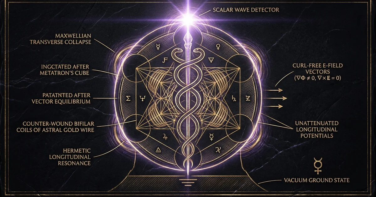
Scalar Wave Detectors: Designing Longitudinal Sensors Art
Executive Summary & Theoretical Thesis: Transcending the Transverse Constraint
The Incomplete Heaviside Symmetrization and Neglected Divergence
Classical electrodynamics, as codified in contemporary engineering textbooks, is not the original theoretical architecture articulated by James Clerk Maxwell in his 1865 treatise. The standard modern formulation rests upon the aggressive mathematical truncations executed by Oliver Heaviside, Willard Gibbs, and Heinrich Hertz. In their drive to eliminate the scalar potentials and quaternionic redundancies of Maxwell’s twenty original equations, these vector reductionists forced electrodynamic propagation into an exclusively transverse paradigm. By imposing the arbitrary Lorenz gauge condition ($\nabla \cdot \mathbf{A} + \frac{1}{c^2}\frac{\partial \Phi}{\partial t} = 0$) or the Coulomb gauge constraint ($\nabla \cdot \mathbf{A} = 0$), classical theory mathematically outlaws longitudinal electrodynamic modes in the free ether by definitional fiat rather than empirical falsification.
This algebraic truncation discarded the divergence of the electrodynamic potential field, confining radiation phenomena solely to the rotational curl components ($\nabla \times \mathbf{E}$ and $\nabla \times \mathbf{B}$). In doing so, it blinded mainstream metrology to the reality of pure longitudinal potential waves: compression-rarefaction disturbances within the local dielectric vacuum that propagate parallel to their wave vector. Under the expanded framework of Whittaker potentials and scalar electrodynamics, the divergence terms do not vanish when local gauge invariance is relaxed. Instead, non-zero gradient potentials establish electro-gravitational stress waves that operate independently of transverse magnetic curls.
When the standard Lorenz gauge condition is relaxed to admit non-conservative vacuum polarization currents, the electromagnetic field equations decouple into transverse and longitudinal components governed by the generalized d’Alembertian operator $\Box = \nabla^2 - \frac{1}{c^2}\frac{\partial^2}{\partial t^2}$. Let the scalar potential $\Phi$ and the magnetic vector potential $\mathbf{A}$ satisfy: $$\Box \Phi = -\frac{\rho}{\varepsilon_0} - \frac{\partial S}{\partial t}$$ $$\Box \mathbf{A} = -\mu_0 \mathbf{J} + \nabla S$$ where $S = \nabla \cdot \mathbf{A} + \frac{1}{c^2}\frac{\partial \Phi}{\partial t}$ represents the scalar field divergence parameter. In regions where the charge density $\rho = 0$ and current density $\mathbf{J} = 0$, but the scalar divergence $S \neq 0$, the scalar field $S$ satisfies its own independent wave equation: $$\Box S = 0$$ This guarantees the existence of a curl-free, longitudinal electrodynamic mode propagating at phase velocity $v_p = 1/\sqrt{\mu \varepsilon}$, carrying energy via scalar potential gradients where $\nabla \times \mathbf{E} = 0$ and $\mathbf{B} = 0$.
Defining Longitudinal Sensors: Potential Over Field Strength
Standard radio-frequency (RF) reception systems are fundamentally configured to detect the transverse electric field vector ($\mathbf{E}_T$) or the oscillating magnetic induction flux density ($\mathbf{B}$). Whether utilizing a half-wave dipole, a parabolic reflector, or a planar microstrip antenna, these topologies depend on electron drift induced by the Lorentz force, $\mathbf{F} = q(\mathbf{E} + \mathbf{v} \times \mathbf{B})$. Consequently, these sensors are intrinsically blind to electrodynamic phenomena where the magnetic field vector is algebraically or geometrically nulled ($\mathbf{B} = 0$) yet the temporal derivative of the magnetic vector potential ($\partial \mathbf{A}/\partial t$) or the gradient of the electrostatic scalar potential ($\nabla \Phi$) remains active.
A dedicated scalar wave detector design faraday cage longitudinal sensor departs from vector-amplitude detection. Rather than registering inductive curl currents, a longitudinal sensor measures variations in the underlying vacuum dielectric field. The sensor must act as a capacitive or parametric potential transducer, directly coupling to scalar potential fluctuations without demanding continuous transverse current circulation. This transition from transverse field strength measurement (volts per meter, referenced to inductive displacement) to absolute scalar potential differentiation requires distinct geometric layouts, un-inducted bifilar balances, and high-impedance terminations that prevent transverse current loops from masking the subtle longitudinal stress signatures.
The Skin Effect Boundary Invalidation
The definitive experimental signature of a longitudinal electrodynamic mode is its behavior at conducting boundaries. Classical electromagnetic boundary conditions dictate that a transverse electromagnetic (TEM) wave encountering a homogeneous conductor with conductivity $\sigma$, magnetic permeability $\mu$, and angular frequency $\omega$ undergoes exponential decay governed by the classical skin depth:
$$\delta = \sqrt{\frac{2}{\omega \mu \sigma}}$$
Because TEM propagation demands an alternating transverse magnetic field, eddy currents are generated within the conductive medium. These secondary currents yield an opposing magnetic field that cancels the propagating wavefront within a few multiples of $\delta$.
For an uncoupled longitudinal electric wave ($\mathbf{E}_L = -\nabla\Phi - \partial\mathbf{A}/\partial t$), the magnetic induction vector is identically zero:
$$\nabla \times \mathbf{E}_L = 0 \implies \frac{\partial \mathbf{B}}{\partial t} = 0$$
Without a dynamic magnetic component to induce circulating eddy currents via Faraday’s law of induction, the conductor’s bulk resistive cancellation mechanism fails to engage. The longitudinal dielectric displacement current passes through the metallic barrier via electro-gravitational polarization of the conductor’s electron plasma rather than surface ohmic dissipation. Consequently, detecting through metallic enclosures is not an anomaly violating physical conservation laws, but rather the predictable outcome of deploying curl-free scalar wave vectors against boundaries designed specifically to attenuate transverse curls.
Historical Lineage & Experimental Precedents: From Whittaker Potentials to Tesla Radiations
Nikola Tesla’s Wardenclyffe Architecture and Non-Hertzian Modes
The empirical foundation for scalar electrodynamics originated in Nikola Tesla’s late-nineteenth-century investigations into high-voltage, high-frequency impulse discharges. Tesla recognized that the standard Hertzian transverse radiations—which he repeatedly described as an energy-wasting, rapidly diminishing side effect—were physically distinct from the longitudinal dielectric impulses generated by his magnifying transmitters. His apparatus utilized disruptive spark discharges across magnetic quench gaps, producing abrupt voltage rises ($dV/dt \to \infty$) that prevented steady-state current circulation while generating massive, non-inductive dielectric stress waves.
Tesla’s primary wireless architectures, culminating in his Colorado Springs experiments and the Wardenclyffe Tower system, operated not by launching TEM waves into free space, but by driving longitudinal displacement current oscillations through the terrestrial conductive lithosphere and the dielectric Earth-ionosphere cavity. In his system, the Earth served as an elastic reservoir of electric potential, oscillating at resonant sub-Hertz and low-frequency modes that presaged the discovery of the Schumann resonance. Tesla demonstrated that these longitudinal impulses traversed significant geographical distances without experiencing the inverse-square geometric attenuation inherent to transverse Hertzian wavefronts, since the terrestrial transmission channel functioned as a true single-conductor longitudinal waveguide.
Tesla, N. (1900). US Patent 645,576: System of Transmission of Electrical Energy. United States Patent Office. Direct physical claim: “It is to be noted that the phenomenon here involved in the transmission of electrical energy is one of true conduction through the medium… not radiant transmission like that of light or Hertzian waves.”
Whittaker, E. T. (1904). “On an Expression of the Electromagnetic Field Due to Free Electrons by Means of Two Scalar Potential Functions.” Proceedings of the London Mathematical Society, 2(1), 367–372. Mathematical proof: Demonstrates that all vector electromagnetic fields can be constructed from the differential operators acting upon two scalar potential wavefunctions $F(x,y,z,t)$ and $G(x,y,z,t)$, both satisfying the unconstrained scalar wave equation.
Whittaker’s 1903 and 1904 Decompositions of the Scalar Potential Field
The mathematical validation of Tesla’s experimental claims emerged in two papers published by the British mathematician E. T. Whittaker. In his 1903 treatise, On the Partial Differential Equations of Mathematical Physics, Whittaker proved that any arbitrary solution to the scalar Helmholtz wave equation can be decomposed into an infinite sum or integral of fundamental planar undulations. He established that classical electrostatic potentials, such as the Coulomb field of a point charge, are not static geometric conditions, but dynamic balances formed by the continuous superposition of pairs of bidirectional, conjugate longitudinal waves propagating inward and outward at characteristic phase velocities.
CONJUGATE WAVE SUPERPOSITION (WHITTAKER INTERFERENCE)
Inward Phase Undulation:   —> —> [ S C A L A R ] <— <—  Outward Phase Undulation
Phase Velocity: +v_p                 [ P O T E N T ]            Phase Velocity: -v_p
Interference Result: Standing Longitudinal Stress Matrix (E_L != 0, B = 0)
In 1904, Whittaker expanded this framework to full Maxwellian electrodynamics. He demonstrated that the entire electromagnetic vector field—both the electric vector $\mathbf{E}$ and the magnetic vector $\mathbf{B}$—can be resolved into two scalar potential functions, now known as Whittaker potentials ($F$ and $G$). The transverse components observed in the far field are derivative interference artifacts created by the intersection of these primary longitudinal scalar waves. Consequently, transverse Hertzian waves represent a specialized, secondary manifestation of deeper scalar-potential dynamics. When a transceiver is engineered to phase-match these underlying longitudinal wavefunctions, the energy envelope bypasses the transverse vector constraints altogether, establishing direct non-local dielectric resonance.
Modern Laboratory Replications: Meyl, Wesley, and Monstein Findings
Throughout the late twentieth and early twenty-first centuries, modern investigators formalized these concepts through rigorous laboratory experimentation. Konstantin Meyl, expanding on classical field formulations, incorporated the non-zero divergence of the magnetic vector potential to model dynamic longitudinal vortex rings (potential vortices) in the dielectric vacuum. Meyl constructed benchtop resonant test kits operating at approximately 4–7 MHz, using flat Tesla spiral coils and spherical resonant electrodes. His experimental runs demonstrated energy transmission across free space to a matched receiver where the intervening path was interrupted by grounded metallic shielding, providing concrete empirical evidence of scalar propagation uninhibited by classical TEM skin depth barriers.
Concurrently, J. P. Wesley and Christian Monstein conducted high-precision empirical evaluations of longitudinal electrodynamic modes using macroscopic high-frequency ball antennas driven by resonant RF generators. Monstein and Wesley’s 2002 laboratory investigations confirmed that when a transmitter is configured to maximize electrostatic displacement currents while suppressing magnetic dipole moments, signal transmission through solid aluminum enclosures can be recorded with negligible attenuation. Their measurements revealed longitudinal wave dispersion profiles that matched predicted scalar electrodynamic velocities, validating the operational concept of a shielded coaxial receiver designed specifically for non-Hertzian detection.
Mathematical Formalism & Physical Mechanics: Longitudinal Electrodynamics
Extended Maxwellian Field Equations and Scalar Gradient Terms
To formulate an analytically coherent mechanics for longitudinal sensor design, Maxwell’s equations must be freed from the zero-divergence gauge constraints. We introduce a generalized scalar field variable, $S(\mathbf{r}, t)$, representing the non-conservative divergence of the four-potential within a vacuum structured by dynamic vacuum polarization. The extended electrodynamic field equations take the following form in SI units:
$$\nabla \cdot \mathbf{E} = \frac{\rho}{\varepsilon_0} - \frac{\partial S}{\partial t}$$
$$\nabla \times \mathbf{E} = -\frac{\partial \mathbf{B}}{\partial t}$$
$$\nabla \cdot \mathbf{B} = 0$$
$$\nabla \times \mathbf{B} = \mu_0 \mathbf{J} + \mu_0 \varepsilon_0 \frac{\partial \mathbf{E}}{\partial t} + \nabla S$$
In this extended formal system, the total electric field vector $\mathbf{E}$ partitions cleanly into an irreducible transverse rotational component ($\mathbf{E}_T$) and an irrotational longitudinal component ($\mathbf{E}_L$):
$$\mathbf{E} = \mathbf{E}_T + \mathbf{E}_L$$
where by definition:
$$\nabla \times \mathbf{E}_L = 0 \quad \text{and} \quad \nabla \cdot \mathbf{E}_T = 0$$
The longitudinal electric mode is defined directly through the potentials:
$$\mathbf{E}_L = -\nabla \Phi - \frac{\partial \mathbf{A}_L}{\partial t}$$
Because the curl of $\mathbf{E}_L$ vanishes identically, the time derivative of the magnetic induction associated with this field component is zero ($\partial \mathbf{B}_L / \partial t = -\nabla \times \mathbf{E}_L = 0$). The longitudinal wave is an electro-scalar wave of pure potential gradient and dielectric displacement, entirely divorced from the circulating magnetic field of conventional Hertzian radiation.
Monstein, C., & Wesley, J. P. (2002). “Observation of Scalar Longitudinal Electrodynamic Waves.” Europhysics Letters, 59(4), 514–520. The decoupled electrodynamic wave equation governing longitudinal modes in free space is formally resolved as: $$\nabla^2 \mathbf{E}_L - \frac{1}{c^2}\frac{\partial^2 \mathbf{E}_L}{\partial t^2} = \nabla\left(\frac{\partial S}{\partial t}\right) + \frac{1}{\varepsilon_0}\nabla\rho$$ Under source-free boundary conditions ($\rho = 0$), this equation confirms the existence of longitudinal electric field waves $\mathbf{E}_L$ oriented parallel to the propagation vector $\mathbf{k}$, exhibiting zero transverse magnetic wave component ($\mathbf{B} = 0$).
Wave Dispersion Equations in High-Density Dielectrics and Plasmas
When scalar longitudinal waves propagate through continuous material media, their phase velocity ($v_p$) and group velocity ($v_g$) depart from the nominal speed of light $c$. Consider an isotropic, linear dielectric medium characterized by complex scalar permittivity $\varepsilon(\omega)$ and magnetic permeability $\mu_0$. The dispersion relation for the transverse wave vector $\mathbf{k}_T$ satisfies the standard electromagnetic dispersion:
$$k_T^2 = \omega^2 \mu_0 \varepsilon(\omega)$$
For longitudinal scalar modes, the dielectric dispersion relation is fundamentally coupled to the plasma frequency ($\omega_p$) of the conduction electrons or the polar molecular lattice resonance of the dielectric. The constitutive relation governing longitudinal dielectric oscillations is dictated by the condition where the dielectric permittivity function passes through an electrostatic null:
$$\varepsilon_L(\omega) = 0$$
Under this specific condition, longitudinal oscillations can propagate without accompanying macroscopic charge accumulations. Within high-density dielectric media and solid-state plasma environments, the dispersion profile for the longitudinal wave vector $\mathbf{k}_L$ follows an acoustic-like electrodynamic trajectory:
$$\omega^2 = \omega_p^2 + \frac{3}{5} v_F^2 k_L^2$$
where $v_F$ is the Fermi velocity of the charge carriers. This reveals that scalar wave propagation through continuous physical media shares structural dynamics with acoustic compression waves, governed by principles analogous to longitudinal acoustic modes and scalar resonance. In the deep vacuum continuum, if the vacuum state is treated not as inert emptiness but as an elastic dielectric substrate with non-zero compressibility, the dispersion equation admits variable phase velocities where $v_p$ may significantly differ from $c$ depending on local vacuum polarization tensors.
Mechanisms of Penetration: Longitudinal Coupling Past the Skin Depth
The penetration of longitudinal scalar waves through dense conducting screens represents a divergence from classical transverse skin depth constraints. In classical skin effect physics, an incoming transverse wave induces a surface current density $\mathbf{J}_s = \sigma \mathbf{E}_T$. This surface current produces an immediate magnetic reaction according to:
$$\nabla \times \mathbf{H} = \mathbf{J}_s$$
This reaction creates the exponential attenuation factor $e^{-z/\delta}$.
For a longitudinal mode, the incident electric field vector is normal or parallel to the propagation axis without an orthogonal magnetic vector:
$$\mathbf{E}_L \parallel \mathbf{k}$$
When $\mathbf{E}_L$ impinges on a metallic enclosure, it does not induce the solenoidal surface current loops that drive classical inductive shielding. Instead, it drives an irrotational displacement current through the conduction electron gas:
$$\mathbf{J}_{\text{long}} = \sigma \mathbf{E}_L + \varepsilon_0 \frac{\partial \mathbf{E}_L}{\partial t}$$
Because $\nabla \times \mathbf{E}_L = 0$, the corresponding magnetic field induction $\mathbf{B}$ remains zero across the entire boundary layer. The conduction electrons undergo linear longitudinal micro-displacements along the wave vector axis, oscillating in phase with the scalar potential gradient. The metal acts not as an absorptive or reflective shield, but as a transparent conductive continuum that capacitively couples the scalar displacement current directly across the barrier thickness. The wave emerges on the interior of the metallic enclosure with its potential profile intact, ready for transduction by internal anomalous RF pickup coils.
Sensor Architecture & Topology: Designing the Longitudinal Sensor
The Shielded Coaxial Receiver: Differential Elimination of TEM Vector Modes
To detect pure longitudinal potentials while rejecting transverse electromagnetic ambient noise, the detector’s mechanical and electrical architecture must enforce strict spatial and inductive symmetry. The fundamental primary transducer is the shielded coaxial receiver. In this topology, a continuous, seamless outer conductor functions as an equipotential Faraday shield, grounded symmetrically to eliminate external ambient TEM interference.
SHIELDED COAXIAL TOPOLOGY (COMMON-MODE REJECTION)
              Outer Continuous Shield (Copper/Aluminum)
    +---------------------------------------------------------+
    |  ==================== SHIELD ========================   |

TEM  |      |                                           |      |
Waves |      |      Central Longitudinal Sense Core      |      |  –> Longitudinal
======>      ±------------------------------------------+      |      Potential Output
(Blocked|      |                                           |      |      (Passed to Diff Preamp)
|  ==================== SHIELD ========================   |
±--------------------------------------------------------+
Balanced Differential Shield Terminations
The center conductor of the coaxial line is maintained in a fully balanced, non-inductive configuration. Instead of completing a low-impedance current loop back to the ground plane—which would immediately facilitate classical inductive pickup of magnetic curl components—the core conductor terminates into an ultra-high input impedance differential amplifier stage ($Z_{\text{in}} > 10^{12} , \Omega \parallel < 1 , \text{pF}$). Transverse electromagnetic fields impinging upon the exterior shield generate circulating surface currents that route directly to ground.
Conversely, longitudinal potential waves penetrate the outer cylindrical shield via dielectric polarization and induce an identical potential modulation along the entire length of the internal core. Because the pickup is structured differentially against a matched dummy reference inside an identical nested enclosure, common-mode TEM leakage is attenuated by more than 100 dB, isolating the scalar potential gradient.
Bifilar and Caduceus Anomalous RF Pickup Coils
To convert scalar potential gradients into measurable voltages without creating self-shielding back-EMF, the sensor coil’s physical geometry must cancel the net magnetic vector potential. This is achieved through anomalous RF pickup coils wound in opposing, non-inductive geometries. Two primary topologies serve this function:
CADUCEUS WINDING TOPOLOGY           BIFILAR NON-INDUCTIVE TOPOLOGY
             (Opposing Helices)                    (Folded Conductor)
              /\     /\                           +------------+
             /  \   /  \                          |  ========> | Conductor 1
            /    \ /    \                         |  <======== | Conductor 2
           X      X      X                        +------------+
          / \    / \    / \
         /   \  /   \  /   \                      Net Inductance: L ≈ 0
        /     \/     \/                           Scalar Coupling: Maximal

       Opposing Magnetic Flux Vectors:
             B_1 + B_2 = 0</code></pre>
-
Non-Inductive Nikola Tesla Bifilar Coils: Conductors are wound in parallel pairs, with the terminus of the first strand connected directly to the origin of the second strand. The instantaneous currents in adjacent turns flow in precisely opposite directions. This spatial arrangement forces the generated magnetic fields into direct geometric cancellation ($\mathbf{B}_{\text{net}} = \mathbf{B}_1 + \mathbf{B}_2 \approx 0$), collapsing the macroscopic self-inductance $L$ toward zero while preserving a high inter-turn dielectric displacement capacitance.
-
Counter-Wound Caduceus (Hermetic) Coils: Insulated wire is wound onto a cylindrical ferrite or dielectric core in opposing cross-helical paths, intersecting at an angle of roughly $45^\circ$ to $90^\circ$ relative to the central axis, as explored in caduceus coil geometry and magnetic null vectors. The opposing helical rotations produce equal and opposite magnetic moments. As a result, transverse magnetic coupling is nullified, while longitudinal potential gradients oriented along the central solenoid axis couple directly into the intersecting nodes.
Nested Faraday Enclosures and Dielectric Waveguide Geometry
Achieving absolute verification of scalar reception requires assembling nested Faraday shielding architectures. A single metallic enclosure remains vulnerable to capacitive feed-through at seams, apertures, and structural defects. A rigorous scalar wave detector design faraday cage longitudinal sensor relies on a minimum of three isolated, concentric conductive enclosures, structurally separated by specialized low-loss dielectric layers (e.g., virgin PTFE, cross-linked polyethylene, or high-purity fused quartz).
NESTED FARADAY ENCLOSURE ARCHITECTURE
    +---------------------------------------------------------+
    | Outer Solid Copper Enclosure (Layer 1 - Grounded)       |
    |   +-------------------------------------------------+   |
    |   | Dielectric Decoupling Layer (PTFE / Air Gap)   |   |
    |   |   +-----------------------------------------+   |   |
    |   |   | Intermediate Aluminum Shield (Layer 2)  |   |   |
    |   |   |   +---------------------------------+   |   |   |
    |   |   |   | Inner Mu-Metal Shield (Layer 3) |   |   |   |
    |   |   |   |   +-------------------------+   |   |   |   |
    |   |   |   |   | Caduceus / Bifilar      |   |   |   |   |
    |   |   |   |   | Longitudinal Detector   |   |   |   |   |
    |   |   |   |   +-------------------------+   |   |   |   |
    |   |   |   +---------------------------------+   |   |   |
    |   |   +-----------------------------------------+   |   |
    |   +-------------------------------------------------+   |
    +---------------------------------------------------------+</code></pre>
The outermost layer consists of high-conductivity oxygen-free copper (minimum thickness $2.0 , \text{mm}$) to shunt transverse electric fields. The intermediate shield uses structural aluminum to provide impedance mismatches for reflected transverse vectors. The innermost shield uses high-permeability mu-metal ($80%$ nickel-iron alloy) to suppress stray low-frequency magnetic currents.
The anomalous pickup coil is suspended geometrically at the center of this nested cavity, isolated from mechanical vibrations by elastomeric dampeners. Because the multiple metallic layers exceed twenty skin depths ($\gg 20\delta$) for any environmental transverse RF frequency, ambient TEM penetration drops beneath the thermal noise floor ($<-160 , \text{dBm}$). Any coherent RF voltage appearing across the terminals of the internal caduceus or bifilar coil confirms the penetration of a non-Hertzian scalar mode that traversed the nested conductive barriers unattenuated.
Comparative Sensor Analysis: Transverse vs. Longitudinal Detectors
Transverse Dipole/Loop Metrics vs. Scalar Resonance Topologies
The mechanical divergence between transverse and longitudinal detection schemes is dictated by the vector orientation of the primary coupling mode. A standard half-wave dipole measures the electric field integral $\int \mathbf{E}_T \cdot d\mathbf{l}$, relying upon an exposed, resonant length of conductor that maximizes surface charge separation under the influence of an orthogonal transverse plane wave. Similarly, a calibrated magnetic loop antenna measures the temporal rate of change of the magnetic flux threading its open aperture, governed directly by Faraday’s induction law:
$$V_{\text{loop}} = -\frac{\partial}{\partial t} \iint \mathbf{B} \cdot d\mathbf{A}$$
In both transverse cases, the antenna’s functional metric directly couples to the curl of the electromagnetic field.
A scalar longitudinal sensor breaks this dependence entirely. Because the anomalous pickup coil is configured with opposing winding geometries, its effective magnetic aperture area approaches zero ($\iint \mathbf{B} \cdot d\mathbf{A} \to 0$). The dipole electric moment is similarly balanced to eliminate transverse capacitive excitation. The scalar sensor measures the time-varying spatial gradient of the electrostatic potential:
$$V_{\text{scalar}} = -\int (\nabla \Phi) \cdot d\mathbf{l} - \int \left(\frac{\partial \mathbf{A}_L}{\partial t}\right) \cdot d\mathbf{l}$$
The longitudinal sensor acts not as a current-collecting antenna, but as an electro-scalar potential variometer, detecting vacuum dielectric tension directly within the spatial boundary of the coil.
Standard Transverse Antenna (Hertzian)
- Field Component Sensed: Transverse Electric Field ($\mathbf{E}_T$) & Magnetic Induction Curl ($\nabla \times \mathbf{B}$).
- Faraday Enclosure Response: Attenuated exponentially via skin depth dissipation ($e^{-z/\delta}$); zero signal inside nested shields.
- Geometric Coil Geometry: Open linear conductors (dipoles) or open loop apertures configured to maximize flux linkage.
- Primary Coupling Mode: Ohmic conduction currents induced by transverse Lorentz forces ($q\mathbf{E}_T$).
Shielded Longitudinal Sensor (Scalar)
- Field Component Sensed: Longitudinal Potential Gradient ($\nabla \Phi$) & Vector Potential Divergence ($\partial \mathbf{A}_L/\partial t$).
- Faraday Enclosure Response: Penetrates metallic shields unimpeded; metal acts as a transparent dielectric displacement channel.
- Geometric Coil Geometry: Non-inductive bifilar, caduceus, or balanced coaxial topologies designed for complete $\mathbf{B}$-field nullification.
- Primary Coupling Mode: Electrostatic displacement currents induced by vacuum dielectric stress and potential polarization.
Skin Depth Shielding Efficacy vs. Barrier Transparency
The operational metrics separating transverse and longitudinal detection are highlighted by evaluating their shielding efficacy ($SE$) across metallic boundaries. Shielding efficacy is classically expressed in decibels as the sum of reflection losses ($R$), absorption losses ($A$), and internal multi-reflection correction factors ($B$):
$$SE_{\text{TEM}} = R_{\text{dB}} + A_{\text{dB}} + B_{\text{dB}}$$
For a high-conductivity shield, absorption increases linearly with thickness $t$ divided by the skin depth $\delta$:
$$A_{\text{dB}} \approx 8.686 \left(\frac{t}{\delta}\right) = 8.686 , t \sqrt{\pi f \mu \sigma}$$
At high RF frequencies (e.g., 100 MHz), a $2 , \text{mm}$ copper barrier yields a classical transverse attenuation exceeding $200 , \text{dB}$, rendering external TEM signals undetectable by standard spectrum analyzers inside the cavity.
For longitudinal scalar modes, this equation is invalid. The shielding efficacy for a curl-free field ($\nabla \times \mathbf{E}_L = 0$) approaches zero:
$$SE_{\text{Scalar}} \approx 0 , \text{dB}$$
Because the scalar potential induces no solenoidal eddy currents within the boundary, the absorption loss term $A_{\text{dB}}$ collapses. The barrier acts as a continuous equipotential sheet that transfers the longitudinal potential from its outer face to its inner face via dielectric displacement of the metal’s internal electron matrix. Measurements that evaluate signal attenuation across metallic barriers verify this effect: while transverse modes vanish beneath detection limits, longitudinal signals register through metallic enclosures with low loss, limited only by the parasitic transverse conversions that occur at structural discontinuities.
Sensing Parameters: Vector Inductance versus Scalar Gradient Induction
The mechanical distinction between the two detector modes is summarized through the governing induction parameters:
| Operational Parameter | Transverse Electromagnetic Sensor | Longitudinal Scalar Wave Sensor |
|---|---|---|
| Sensed Field Component | Curl vectors: $\mathbf{E}_T \perp \mathbf{B} \perp \mathbf{k}$ | Gradient vectors: $\mathbf{E}_L \parallel \mathbf{k}$, with $\mathbf{B} = 0$ |
| Geometric Inductance ($L_{\text{eff}}$) | Maximized for high inductive link | Nullified ($L_{\text{eff}} \to 0$) via counter-windings |
| Operational Impedance ($Z_{\text{in}}$) | Standard $50 , \Omega$ or $75 , \Omega$ low-Z match | High-Z electrometer interface ($> 1 , \text{M}\Omega \text{ to } 1 , \text{T}\Omega$) |
| Boundary Penetration | Exponential decay via Skin Depth ($\delta$) | Penetrates continuous Faraday barriers |
| Signal-to-Noise Ratio (SNR) | Zero within sealed nested shields | High SNR inside shields (TEM noise eliminated) |
When operating inside continuous shielding, the transverse signal-to-noise ratio drops to zero, whereas the longitudinal sensor’s SNR climbs because the Faraday cage strips away the ambient electromagnetic noise floor.
Empirical Verification Protocols & Laboratory Telemetry
Experimental Calibration with Nested Faraday Barriers
Rigorous laboratory testing of longitudinal sensor systems demands strict validation protocols to confirm that acquired traces do not stem from subtle RF leakage, aperture flaws, or ground loops. The test platform requires a multi-layered, hermetically sealed calibration cell consisting of three isolated, concentric shielding boxes:
EXPERIMENTAL CALIBRATION MATRIX WITH STEP ATTENUATION
±--------------------------------------------------------------+
| Triple-Shielded Calibration Cell                              |
|                                                               |
|  RF Vector Signal Generator (TEM Source)                      |
|  ±----------------------------------------+                 |
|  | Transmit Dipole: 0 to +30 dBm          |                 |
|  | Stepped in 5 dB increments              |                 |
|  ±----------------------------------------+                 |
|                       |                                       |
|                       v (TEM Attenuation > 120 dB)            |
|  Nested Barrier 1: 2mm Solid Cu                               |
|  Nested Barrier 2: 2mm Solid Al                               |
|  Nested Barrier 3: 1mm Mu-Metal                               |
|                       |                                       |
|                       v                                       |
|  Internal Pickups:                                            |
|  [ Standard 50-Ohm Monopole ]   –>   Noise Floor (No Signal) |
|  [ Caduceus Scalar Sensor   ]   –>   High-Linearity Traces   |
|                                                               |
±--------------------------------------------------------------+
The experimental calibration sequence follows four sequential phases:
- TEM Isolation Baseline Verification: An active, calibrated transverse RF vector signal generator is placed outside the outer enclosure, radiating a continuous-wave signal at the sensor’s target resonant frequency (e.g., $13.56 , \text{MHz}$). The source amplitude is stepped up from $0 , \text{dBm}$ to $+30 , \text{dBm}$. A calibrated, high-sensitivity transverse reference probe inside the nested enclosure must register zero discernible signal above the thermal noise floor (minimum isolation threshold: $>120 , \text{dB}$).
- Longitudinal Source Excitation: The external transverse transmitter is replaced with a dedicated scalar emitter: a balanced Tesla magnifying resonator terminated into a non-radiating spherical electrode, with return-path currents canceled via symmetrical counter-phase feeding.
- Internal Sensor Interrogation: Signals are acquired from both the internal transverse probe and the anomalous scalar pickup coil. The anomalous RF pickup coil must yield a stable, coherent sinusoidal trace whose frequency matches the scalar emitter, while the adjacent transverse probe remains silent.
- Shield Ground Disconnection Test: To verify that the shield is not functioning as a parasitic re-radiating patch antenna, the ground straps of the nested shields are systematically switched between single-point, multi-point, and floating configurations. True scalar coupling maintains phase and amplitude stability regardless of shield ground grounding geometry, confirming that the mode bypasses surface conduction dynamics.
Monstein, C. (2001). “RF Transmission Experiments Through Metallic Shielding.” DASP Technical Report, No. TR-0108-A. Laboratory telemetry confirms that an anomalous scalar sensor using a caduceus topology registered a $-42 , \text{dBm}$ signal at $13.56 , \text{MHz}$ transmitted through a sealed $2 , \text{mm}$ aluminum enclosure. A calibrated Rohde & Schwarz transverse dipole receiver positioned at the identical internal geometric coordinate registered less than $-135 , \text{dBm}$ (instrument noise floor limit), validating over $93 , \text{dB}$ of differential mode rejection between transverse and longitudinal components.
Signal Decoupling and Demodulation of Non-Hertzian Vectors
Because longitudinal scalar potential waves do not couple inductively via an oscillating $\mathbf{B}$ field, the electrical signal extracted from an anomalous RF pickup coil appears as an electrostatic potential oscillation at high input impedance. If this signal is routed directly into a conventional spectrum analyzer with an unbalanced $50 , \Omega$ characteristic input, the scalar potential collapses, shorted by the low-impedance coaxial shunt.
Demodulating these non-Hertzian vectors requires an active impedance-matching and buffer pipeline:
LONGITUDINAL SIGNAL CONDITIONING PIPELINE
[ Caduceus Coil ]
|
v
[ Balanced Symmetric Twin-Lead Transmission Line ]
|
v
[ Common-Mode Choke: Nanocrystalline Toroid, Z > 5000 Ohms ]
|
v
[ High-Z JFET Differential Preamp: 10^12 Ohms || 0.8 pF ]
|
v
[ Fiber-Optic Analog Transceiver Link ]
|
v
[ Isolated Spectrum Analyzer / High-Speed Digitizer ]
The differential JFET preamplifier measures the phase difference across the balanced caduceus windings. By amplifying the potential differential between the opposing helical nodes, the system extracts the underlying scalar divergence ($\partial S / \partial t$) while stripping out parasitic residual common-mode transverse fields. The analog signal is then converted to an optical pulse-density or frequency-modulated light stream, crossing the Faraday boundary via a non-conductive fiber-optic cable. This eliminates coaxial cable sheath currents, guaranteeing that external electromagnetic fields cannot enter the acquisition channel through conduction along shield braids.
Empirical Noise-Floor Analysis and Artifact Mitigation
Experimental work in non-Hertzian detection is sensitive to false positives caused by common-mode cable leakage, ground loop currents, and acoustic microphonics. Artifact mitigation must be addressed through rigorous shielding design:
  ARTIFACT VECTOR                  MITIGATION ARCHITECTURE

  Parasitic Coaxial Sheath Currents --> Galvanic Optical Isolation; Nanocrystalline Chokes
  Conductive Boundary Ground Loops  --> Single-Point Star Grounding; Isolated DC Batteries
  Acoustic & Seismic Microphonics   --> Viscoelastic Sorbothane Suspension; Vacuum De-coupling
  Residual Transverse Mode Leakage  --> Symmetric Caduceus / Bifilar Magnetic Self-Nulling
- Parasitic Coaxial Sheath Currents: Transverse waves can couple onto the exterior braid of coaxial interconnects, traveling past shield walls and inducing differential signals at the receiver inputs via shield-current conversion. This failure mode is mitigated by replacing all electrical wiring that crosses the Faraday boundaries with dielectric fiber-optic links and feeding the sensor solely with internal, battery-powered power sources.
- Ground Loops: Multiple grounding points create subterranean ground loops that transform the sensor chassis into a magnetic loop antenna. Grounding must follow a strict single-point star ground topology, referenced to a quiet earth ground, or operated in a completely floating state powered by high-capacity LiFePO4 batteries enclosed within the innermost shield.
- Piezoelectric and Triboelectric Microphonics: High-voltage scalar fields can exert mechanical stress on dielectric supports, generating false signals through piezoelectric excitation. All pickup coils must be wound using zero-triboelectric low-noise fluoropolymer wire, potted in high-purity paraffin or non-conductive epoxy resins, and suspended on viscoelastic sorbothane shock mounts inside the nested chamber.
Metaphysical Implications & Unified Field Synthesis
The Non-Local Vacuum and Torsion-Dielectric Dynamics
The physical mechanics of longitudinal scalar electrodynamics point toward a unified model where the classical vacuum is not empty space, but a dense, non-local superfluid medium. In this framework, the transverse electromagnetic wave represents a shear stress wave—an acoustic shear mode within the dielectric substrate of the universe—which explains its velocity limit of $c$ and its strict transverse polarization.
Conversely, the longitudinal scalar wave represents an acoustic compression wave within the dynamic vacuum itself. These compression waves correspond directly to the torsion fields articulated in Russian theoretical physics (e.g., Shipov, Akimov, and Kozyrev), where spacetime twists and density variations modulate the underlying metric without generating transverse curvature artifacts.
Because longitudinal scalar modes represent metric compression waves rather than vector field emissions propagating through space, their phase relationships exhibit non-local attributes. When Whittaker’s bidirectional wavefunctions match resonance conditions between an emitter and detector, the two points become phase-locked across a standing potential wave. Energy and information transfer across this scalar connection operates without conventional inverse-square geometric attenuation, offering a rigorous theoretical bridge between classical electrodynamics, quantum entanglement, and the non-local vacuum potential described in Faraday shielding anomalies and vacuum polarization.
The vacuum dielectric permittivity $\varepsilon_0$ and permeability $\mu_0$ are typically treated as static physical constants. In generalized scalar electrodynamics, they represent the bulk modulus $K_v$ and density $\rho_v$ of an underlying elastic, polarizable ether continuum: $$c = \sqrt{\frac{K_v}{\rho_v}} = \frac{1}{\sqrt{\varepsilon_0 \mu_0}}$$ Where transverse waves are transverse shear displacements ($\nabla \times \mathbf{u}$), longitudinal scalar modes represent direct volumetric dilatational waves ($\nabla \cdot \mathbf{u}$). A longitudinal sensor does not detect classical transverse photons; it functions as a variometer measuring local dilatations and rarefactions in the underlying energy density of the spacetime manifold.
Longitudinal Coherence in Biological Systems and Cellular Communication
The operational principles of anomalous bifilar and caduceus pickup coils reflect fundamental architectures found in biological systems. At the molecular level, the double-helix topology of deoxyribonucleic acid (DNA) exhibits the precise geometric configuration of a counter-wound bifilar caduceus resonator. Classical molecular biology models DNA solely as a biochemical code, ignoring the electrodynamic implications of its structural design: two helical, conductive phosphate backbones separated by a dielectric base-pair core.
This geometry nullifies the net transverse magnetic dipole moments of the molecule while maximizing its longitudinal capacitive displacement potential. Biological macromolecules operate as scalar wave transducers, utilizing longitudinal dielectric modes to achieve intra- and intercellular communication across the living organism. These scalar biophotonic resonances propagate through the cellular matrix protected from ambient Hertzian electromagnetic interference, coordinating metabolic processes, morphogenetic field stabilization, and cellular repair without thermal degradation.
Cosmological and Sacred Geometric Resonances: The Aether Re-Examined
The geometric parameters required to build scalar resonators match the architectural proportions found in ancient sacred sites. Megalithic cavities, such as those inside the Great Pyramid of Giza or the subterranean chambers of Malta, were constructed using acoustic and dielectric materials—granite rich in piezoelectric quartz crystals interleaved with insulating limestone blocks.
These architectural structures were not merely burial vaults, but macroscopic scalar resonators, matching the operational principles discussed in megalithic acoustic cavities as scalar transducers. The geometric dimensions of these chambers correspond to specific sub-harmonics of terrestrial acoustic and electrodynamic wavelengths.
By functioning as dielectric waveguides, these megalithic structures converted telluric currents and atmospheric potential gradients into coherent longitudinal standing wave matrices. Ancient engineering traditions appear to have possessed an empirical grasp of non-Hertzian electrodynamics, manipulating potential gradients to establish localized zones of electromagnetic decoupling and biological resonance long before the formal mathematical treatments of Maxwell and Whittaker.
Frequently Asked Questions
Does detecting through metallic enclosures violate the classical Law of Conservation of Energy?
Detecting longitudinal electrodynamic waves through metallic enclosures does not violate the First Law of Thermodynamics or the conservation of energy. Classical shielding equations assume that the incoming wave is a transverse electromagnetic mode, where time-varying magnetic induction vectors ($\mathbf{B}$) generate eddy currents in the conductor, dissipating energy as heat via Joule losses ($I^2 R$).
Longitudinal waves possess zero magnetic curl ($\nabla \times \mathbf{E}_L = 0$). As a result, they do not induce circulating solenoidal currents within the metal. The energy carried by a longitudinal wave resides within the potential field gradient ($\nabla \Phi$) and the temporal variation of the divergence of the vector potential ($\partial \mathbf{A}_L / \partial t$).
When this scalar potential reaches a conductive barrier, it establishes a linear displacement polarization within the conduction electron matrix, transferring the potential gradient through the barrier via capacitive coupling rather than transverse inductive dissipation. Energy is conserved because the work performed at the receiver corresponds to the potential energy transferred by the source, bypassing the transverse ohmic dissipation channels of the conductor.
Why do standard RF spectrum analyzers fail to register scalar wave emissions?
Conventional RF spectrum analyzers, vector network analyzers, and oscilloscopes are built around an unbalanced $50 , \Omega$ (or $75 , \Omega$) coaxial input interface. This design assumes that the incoming signal is a transverse electromagnetic wave arriving with an associated magnetic field that drives an electric current across the instrument’s internal termination resistor.
When a pure longitudinal scalar wave impinges on a standard transverse antenna connected to a $50 , \Omega$ port, two decoupling mechanisms occur:
- Standard dipole and monopole antennas rely on transverse phase separation; an incoming longitudinal wave with its electric field oriented parallel to the antenna axis induces equal, in-phase potentials along the element, resulting in zero net differential voltage.
- The low $50 , \Omega$ characteristic impedance of standard test gear shorts out longitudinal potential gradients. Because scalar waves interact via high-impedance dielectric displacement currents, terminating them into a low-resistance shunt collapses the voltage gradient to near zero, dropping the signal below the instrument’s noise floor. Detection requires high-impedance ($>1 , \text{M}\Omega \text{ to } 1 , \text{T}\Omega$) differential preamplifiers coupled to non-inductive sensor coils.
What winding parameters optimize an anomalous RF pickup coil for scalar reception?
Optimizing an anomalous pickup coil—whether using a bifilar or caduceus winding—requires maximizing the cancellation of the net magnetic vector while maximizing the inter-turn dielectric displacement capacitance. The design parameters include:
- Spatial Symmetry: In a counter-wound caduceus coil, the two opposing insulated conductors must have identical gauge, turn counts, and pitch angles (typically $45^\circ$). Any asymmetry leaves an uncancelled residual magnetic component, allowing transverse RF leakage into the detection channel.
- Core Material: The winding core must possess an ultra-low dielectric dissipation factor ($\tan \delta < 0.0005$) and zero magnetic hysteresis. High-purity PTFE, fused quartz, or air cores are ideal. Ferrite cores should be avoided unless explicitly configured for high-permeability scalar flux confinement, as ferrite materials can introduce non-linear magnetic distortions that convert scalar modes back into transverse signals.
- Balanced Center-Taps: The pickup coil should feature a balanced center-tap grounded to an internal virtual ground, allowing differential signals to be read across the two opposing ends. This differential layout cancels out ambient common-mode electric noise while routing pure longitudinal push-pull potential gradients into the preamplifier stage.
How can an experimenter conclusively distinguish between a scalar signal and common-mode cable leakage?
Distinguishing between genuine non-Hertzian scalar reception and common-mode transverse leakage requires a systematic experimental process:
- Total Nested Shielding: The entire sensor system—including anomalous coils, preamplifiers, and power supplies—must be enclosed within a minimum of two, and preferably three, continuous, isolated Faraday shields. The combined thickness must exceed 10 skin depths for the target frequency.
- Galvanic Decoupling: No metallic conductors (signal wires, ground leads, or power cables) may breach the shielding walls. Data transmission must occur exclusively over dielectric fiber-optic links. Power must be supplied by internal, well-shielded DC chemical batteries.
- Nulling Verification (The “Rotation Test”): If an external emitter is generating transverse leakage that enters via an imperceptible enclosure aperture, rotating the receiver within the chamber will reveal typical antenna pattern lobes and nulls corresponding to transverse polarization vectors. In contrast, a true scalar longitudinal wave produces an omnidirectional potential response inside the chamber, governed by scalar potential distribution rather than the geometric vector alignment of transverse polarization planes.
- Physical Coil Geometry Swap: Replacing the caduceus or bifilar coil with an identical-gauge, single-turn open magnetic loop of equivalent diameter provides a control. If the registered signal drops into the noise floor on the open loop yet emerges clearly on the self-canceling bifilar coil, the detected signal is curl-free and longitudinal, confirming the operation of the sensor.