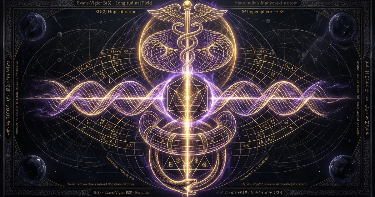
Lost Symmetries: O(3) and SU(2) Higher Electrodynamics

Executive Summary & Theoretical Thesis: Transcending the U(1) Consensus

The Structural Deficiencies of the Standard Abelian U(1) Framework

Classical electrodynamics, as codified in the contemporary Maxwell-Heaviside paradigm, rests on the fundamental postulate that the electromagnetic gauge field is mediated by an Abelian unitary symmetry group, designated as $U(1)$. In this formulation, the four-potential $A_\mu = (\phi/c, -\mathbf{A})$ defines a connection on a principal bundle whose fiber is the one-dimensional circle group. A structural consequence of this Abelian geometry is that the gauge group generators commute: $[T_a, T_b] = 0$. Consequently, the field strength tensor $F_{\mu\nu} = \partial_\mu A_\nu - \partial_\nu A_\mu$ contains purely linear differential terms, precluding photon-photon self-interaction in the classical vacuum. Under these $u1\text{ symmetry limitations}$, the photon behaves as a non-self-interacting, uncharged vector boson whose propagation in free space is strictly transverse, as constrained by the transversality condition $\nabla \cdot \mathbf{B} = 0$ and the radiation gauge $\nabla \cdot \mathbf{A} = 0$.

This mathematical architecture artificially extinguishes longitudinal degrees of freedom from the physical vacuum. By demanding that the electromagnetic gauge connection exist solely within an isotropic, flat $U(1)$ bundle, the standard model of classical electrodynamics dismisses longitudinal electric modes, finite vacuum polarizabilities, and axial magnetic fields as non-physical gauge artifacts. However, this truncation restricts the capacity of field theory to describe extreme non-linear phenomena. When intense electromagnetic radiation interacts with macroscopic structures or non-linear media, the linear superposition principle breaks down. The suppression of longitudinal field components and non-Abelian vacuum topologies has generated persistent theoretical discrepancies between experimental observations in non-linear optics—such as the Inverse Faraday Effect—and the foundational assumptions of classical vacuum electrodynamics. Exploring these potential modes requires re-evaluating the role of the scalar potential and longitudinal modes within extended gauge frameworks.

Topological Fiber Bundles and Higher Gauge Manifolds

To transcend the constraints of the $U(1)$ framework, the underlying base manifold $M$ must be coupled to non-Abelian Lie groups possessing non-trivial geometric curvature. When electrodynamics is formulated over higher-order symmetry groups such as $SU(2)$ (the double cover of the three-dimensional rotation group) or $O(3)$ (the full orthogonal group in three dimensions), the principal fiber bundle $P(M, G)$ acquires intrinsic non-Abelian curvature. Under a non-Abelian Lie algebra $\mathfrak{g}$, the gauge connection 1-form is matrix-valued: $\mathbf{A} = A_\mu^a T_a dx^\mu$, where $T_a$ are the generator matrices satisfying the non-trivial commutation relation $[T_a, T_b] = i C_{ab}^c T_c$, with $C_{ab}^c$ denoting the structure constants of the group.

The transition to an $SU(2)$ or $O(3)$ internal symmetry immediately alters the geometric behavior of the gauge connection. The field strength 2-form $\mathbf{F} = d\mathbf{A} - ig \mathbf{A} \wedge \mathbf{A}$ acquires a non-linear term governed by the Lie bracket. In tensor notation, this manifests as:

$$F_{\mu\nu}^a = \partial_\mu A_\nu^a - \partial_\nu A_\mu^a + g \epsilon^a_{\ bc} A_\mu^b A_\nu^c$$

where $g$ represents an internal coupling parameter and $\epsilon^a_{\ bc}$ is the totally antisymmetric Levi-Civita tensor. This mathematical extension shifts the physical vacuum from a passive, linear spatial background to an active geometric continuum possessing self-coupling capabilities. Within this topological framework, electromagnetic fields exhibit rich vacuum structures, including instanton sectors, non-trivial winding numbers, and topologically protected field configurations that naturally emerge from the underlying geometry. Such global topological properties provide an analytical link to non-local field interactions, directly informing modern investigations into Aharonov-Bohm vacuum topologies where potential configurations govern quantum phase behavior independent of localized classical forces.

The Core Postulate of Non-Abelian Photon Interactions

The physical postulate unifying non-Abelian electrodynamics is that circularly polarized electromagnetic radiation inherently possesses non-Abelian gauge attributes. In standard optics, circular polarization is treated merely as the phase-quadrature superposition of two orthogonal, transverse linear modes within a $U(1)$ framework. Conversely, non-Abelian electrodynamics recognizes that the rotation of the electric and magnetic vector fields in the transverse plane traces an intrinsic spatial vorticity. In the formalisms developed by Myron Evans and Jean-Pierre Vigier, this cyclic rotation is identified as an explicit physical manifestation of the $O(3)$ rotation group acting in field space.

Under this premise, the interaction of transverse electromagnetic conjugate components yields a phase-independent, real, physical magnetic flux density oriented along the axis of propagation: the Evans $B^{(3)}$ field. Unlike standard transverse radiation fields, which oscillate sinusoidally and time-average to zero over an optical cycle, the postulated $B^{(3)}$ field is a non-vanishing, static axial magnetic field in the vacuum. It is generated through the non-Abelian commutator bracket of the transverse conjugate fields:

$$\mathbf{B}^{(1)} \times \mathbf{B}^{(2)} = i B^{(0)} \mathbf{B}^{(3)*}$$

This non-vanishing axial vector represents an intrinsic, gauge-invariant manifestation of vacuum non-linearity. Extending Maxwell’s equations through $O(3)$ and $SU(2)$ internal symmetries bridges classical optics and Yang-Mills gauge theories, demonstrating that the transverse plane waves of classical mechanics are asymptotic reductions of a non-linear gauge manifold capable of sustaining longitudinal vacuum modes.

Historical Lineage & Experimental Precedents: The Suppressed Vector Lineage

From Maxwell’s Quaternions to the Heaviside-Gibbs Truncation

The conceptual limitations of contemporary electromagnetic theory trace back to the mathematical restructuring of James Clerk Maxwell’s original theory. In his definitive 1865 and 1873 publications, Maxwell formulated the laws of electrodynamics utilizing Hamilton’s associative, non-commutative biquaternion algebra. Maxwell’s original synthesis encompassed twenty distinct equations containing twenty scalar variables, intentionally designed to preserve both the scalar and vector potentials as fundamental physical entities. Central to this quaternion architecture was the electromagnetic momentum field—designated by Maxwell as the vector potential $\mathbf{A}$—and its conjugate scalar component $\psi$, which Maxwell treated not as mathematical conveniences, but as foundational indicators of the local state of stress and displacement within the underlying electromagnetic continuum.

During the late nineteenth century, Oliver Heaviside, Josiah Willard Gibbs, and Heinrich Hertz undertook an aggressive condensation of Maxwell’s treatise. Viewing quaternionic analysis as unnecessarily abstract and computationally inefficient for resolving telegraphic transmission challenges, Heaviside replaced the quaternionic operators with modern vector calculus. In doing so, Heaviside reduced the original twenty scalar equations to the canonical four vector equations widely taught today. This reduction achieved significant mathematical efficiency, but it systematically removed the longitudinal scalar wave dynamics and potential-dependent degrees of freedom present in Maxwell’s original texts. The historical implications of this mathematical excision are analyzed in detail within the study of Heaviside quaternions and the lost Maxwell equations.

   Original Maxwell Formulation (1865)
   [ 20 Equations in 20 Variables ]
   [ Quaternionic Vector/Scalar Potentials ]
                   │
                   ▼  Heaviside-Gibbs Truncation (1880s)
   Standard Vector Electrodynamics
   [ 4 Vector Equations, Transverse-Only ]
   [ Potentials Demoted to Mathematical Gauges ]
                   │
                   ▼  Harmuth, Evans, Barrett Re-Evaluation (1980s–1990s)
   Higher Symmetry Electrodynamics
   [ Non-Abelian O(3)/SU(2) Gauge Architectures ]
   [ Restoration of Vacuum Longitudinal Potentials ]

The consequences of this truncation were highlighted by Henning F. Harmuth in his foundational critiques regarding information theory and velocity dispersion in Maxwellian electrodynamics (Harmuth, 1986). Harmuth demonstrated that Heaviside’s transverse equations enforce an infinite phase velocity for zero-frequency spectral components and fail to properly describe the propagation of non-sinusoidal, transient electromagnetic signals without violating causality constraints. By eliminating the longitudinal components and scalar field terms inherent to quaternion mechanics, the vector-analytic consensus created a framework unable to process non-zero longitudinal divergences in non-linear media without inserting ad-hoc phenomenological parameters.

The Discovery of the Inverse Faraday Effect (IFE)

The earliest experimental challenge to the strictly linear, transverse $U(1)$ gauge paradigm emerged in the mid-1960s with the empirical discovery of the Inverse Faraday Effect (IFE). In 1965, J. P. van der Ziel, P. S. Pershan, and L. D. Malmstrom demonstrated that when an intense pulse of circularly polarized optical radiation traverses a non-absorbing diamagnetic material, it induces an internal, macroscopic, time-invariant magnetic moment aligned along the optical wave-vector $\mathbf{k}$.

In standard optics, this induced static magnetization $M_z$ is phenomenologically parameterized via a third-order non-linear optical susceptibility tensor $\chi^{(3)}_{ijk}(-\omega; \omega, -\omega, 0)$:

$$M_z = \frac{i}{4\pi} \chi^{(3)}_{xyz} E_x(\omega) E_y^*(\omega)$$

While this phenomenological formulation adequately captures the bulk material response of diamagnetic glasses and rare-earth-doped crystals at moderate laser power densities ($10^6 - 10^8 \text{ W/cm}^2$), it characterizes the magnetization entirely as a secondary induced electronic current loop inside the atomic electron cloud. It assigns no structural capacity for magnetization directly to the electromagnetic field itself.

The standard approach encounters theoretical difficulties when explaining why the proportionality factor between field intensity and induced magnetic moment remains remarkably stable across disparate material phases, including low-density gaseous plasmas where atomic bound states are stripped. The experimental realization of the Inverse Faraday Effect indicated that circularly polarized radiation carries an intrinsic, field-theoretic angular momentum capable of coupling directly to the vacuum state, pointing toward the need for a non-linear revision of the underlying gauge symmetry.

The Barrett and Evans Formulations of Higher Symmetry Electrodynamics

During the 1990s, theoretical physicists Terence W. Barrett and Myron W. Evans independently recognized that the limitations of the $U(1)$ framework in resolving non-linear optical phenomena could be resolved by embedding the electromagnetic field within higher-dimensional non-Abelian symmetry algebras. Barrett approached the problem through the lens of topological physics and differential geometry. In his 1993 monograph, Electromagnetic Phenomena Not Explained by Maxwell’s Equations, Barrett formulated an $SU(2)$ non-Abelian electrodynamic framework to explain anomalies in dielectric polarization, high-frequency energy transfer, and the conditioning of electromagnetic radiation. He demonstrated that by expanding the gauge symmetry to $SU(2)$, the electromagnetic field supports topological invariants, non-transverse boundary waves, and phase-dependent interferences that standard $U(1)$ equations cannot accommodate.

Simultaneously, Myron W. Evans, building on the theoretical physics foundations laid by Jean-Pierre Vigier and Louis de Broglie, introduced the $O(3)$ higher-symmetry electrodynamic architecture. Evans contended that the transverse plane-wave solutions of the Maxwellian field represent only an incomplete projection of a broader three-dimensional rotation group. By formalizing the cyclic relations between the complex conjugate transverse components $\mathbf{B}^{(1)}$ and $\mathbf{B}^{(2)}$ and the longitudinal vector $\mathbf{B}^{(3)}$, Evans introduced a non-Abelian gauge theory wherein the photon’s own field operations exhibit non-vanishing commutators in free space. The resulting Evans-Vigier formulation provided a direct mechanism for the Inverse Faraday Effect: rather than requiring an atomic dielectric medium to establish non-linear magnetization via third-order susceptibilities, the light beam intrinsically delivers an axial, phase-independent magnetic field density—the Evans $B^{(3)}$ field—as an inherent geometric feature of the vacuum field itself.

Mathematical Formalism & Physical Mechanics: The SU(2) and O(3) Lie Algebras

The Non-Abelian Field Strength Tensor and Gauge Covariance

The non-Abelian extension of classical electrodynamics is rooted in the mathematical formalism originally established by Chen-Ning Yang and Robert L. Mills in 1954 for the conservation of isotopic gauge invariance. Let $G$ represent an internal compact non-Abelian Lie group, specifically $SU(2)$ or its adjoint representation $SO(3) \cong O(3)$, associated with the Lie algebra $\mathfrak{g}$. The generators of the algebra, denoted $T_a$ ($a \in {1, 2, 3}$), obey the foundational commutation relations:

$$[T_a, T_b] = i \epsilon_{abc} T_c$$

where $\epsilon_{abc}$ is the completely antisymmetric Levi-Civita symbol. The gauge-covariant derivative acting on a matter field or multiplet $\psi$ in the fundamental representation is defined as:

$$D_\mu = \partial_\mu - ig A_\mu^a T_a$$

where $g$ denotes the gauge coupling constant and $A_\mu^a$ represents the matrix-valued gauge connection 1-form. The associated field strength tensor $\mathbf{F}{\mu\nu} = F{\mu\nu}^a T_a$ is computed directly through the commutator of the covariant derivatives:

$$[D_\mu, D_\nu] = -ig F_{\mu\nu}^a T_a$$

Expanding this commutator yields the explicit non-Abelian field strength tensor:

$$F_{\mu\nu}^a = \partial_\mu A_\nu^a - \partial_\nu A_\mu^a + g \epsilon^a_{\ bc} A_\mu^b A_\nu^c$$

The presence of the quadratic non-Abelian term $g \epsilon^a_{\ bc} A_\mu^b A_\nu^c$ marks the departure from linear Maxwellian mechanics. The gauge transformation of the field strength tensor under an element $U(x) = \exp(i \theta^a(x) T_a) \in G$ obeys the adjoint representation:

$$\mathbf{F}{\mu\nu} \to U \mathbf{F}{\mu\nu} U^{-1}$$

which ensures that the Yang-Mills Lagrangian density:

$$\mathcal{L} = -\frac{1}{4} F^{a\mu\nu} F_{\mu\nu}^a$$

remains strictly gauge invariant. The Euler-Lagrange equations applied to this Lagrangian yield the non-Abelian field equations of motion:

$$D_\mu F^{a\mu\nu} = \partial_\mu F^{a\mu\nu} + g \epsilon^a_{\ bc} A_\mu^b F^{c\mu\nu} = j^{a\nu}$$

where $j^{a\nu}$ represents the external matter current density. Crucially, the term:

$$J_{\text{self}}^{a\nu} = -g \epsilon^a_{\ bc} A_\mu^b F^{c\mu\nu}$$

functions as an intrinsic, vacuum self-interaction current. In non-Abelian electrodynamics, the vacuum behaves as a self-sourcing medium; the gauge fields themselves carry non-Abelian gauge charge, driving non-linear vacuum self-focusing, beam confinement, and the generation of longitudinal magnetic components without requiring external material sources.

The Cyclic Commutator Relations of the Evans B-Field Triad

The structural manifestation of non-Abelian electrodynamics in optical systems is codified by the Evans $B$-field triad. In classical Cartesian coordinates, an elliptically or circularly polarized electromagnetic wave propagating along the $z$-axis is characterized by transverse electric and magnetic fields oscillating in the $x$-$y$ plane. To analyze the underlying $O(3)$ Lie group symmetry, Evans projected these field vectors into a complex circular basis defined by the orthogonal unit vectors:

$$\mathbf{e}^{(1)} = \frac{1}{\sqrt{2}}(\mathbf{i} - i\mathbf{j}), \quad \mathbf{e}^{(2)} = \frac{1}{\sqrt{2}}(\mathbf{i} + i\mathbf{j}) = \mathbf{e}^{(1)*}, \quad \mathbf{e}^{(3)} = \mathbf{k}$$

These unit vectors satisfy the cyclical geometric cross-product relations:

$$\mathbf{e}^{(1)} \times \mathbf{e}^{(2)} = i \mathbf{e}^{(3)}, \quad \mathbf{e}^{(2)} \times \mathbf{e}^{(3)} = i \mathbf{e}^{(1)}, \quad \mathbf{e}^{(3)} \times \mathbf{e}^{(1)} = i \mathbf{e}^{(2)*}$$

In the $O(3)$ electrodynamic paradigm, the physical magnetic field vector is represented as a multiplet spanning these three basis vectors:

$$\mathbf{B} = \mathbf{B}^{(1)} \mathbf{e}^{(1)} + \mathbf{B}^{(2)} \mathbf{e}^{(2)} + \mathbf{B}^{(3)} \mathbf{e}^{(3)}$$

where the transverse components correspond to the dynamic, conjugate radiative fields:

$$\mathbf{B}^{(1)} = \frac{B^{(0)}}{\sqrt{2}}(\mathbf{i} - i\mathbf{j}) e^{i(\omega t - \kappa z)}, \quad \mathbf{B}^{(2)} = \frac{B^{(0)}}{\sqrt{2}}(\mathbf{i} + i\mathbf{j}) e^{-i(\omega t - \kappa z)} = \mathbf{B}^{(1)*}$$

with $B^{(0)}$ denoting the peak field amplitude, $\omega$ the angular frequency, and $\kappa = \omega/c$ the wave-number.

In an Abelian $U(1)$ framework, the cross product of two fields propagating in the same direction merely yields an instantaneous Poynting-like vector flux; it cannot source a time-invariant static field along the propagation axis in free space without invoking macroscopic material polarization charges. In $O(3)$ electrodynamics, the cyclic commutator directly demands that a real, phase-independent, time-invariant axial magnetic field $\mathbf{B}^{(3)} = B^{(0)} \mathbf{k}$ exists simultaneously in the vacuum alongside the propagating transverse modes.

Topological Solitons, Instanton Sectors, and Beltrami Fields

When electrodynamics is elevated to an $SU(2)$ or $O(3)$ gauge symmetry, the vacuum supports non-trivial topological configurations that are unstable or mathematically forbidden in linear $U(1)$ theory. Among the most significant of these configurations are Beltrami fields—vector fields where the curl of the field is everywhere collinear to the field itself:

$$\nabla \times \mathbf{B} = \alpha \mathbf{B}$$

where $\alpha$ is a scalar function or constant parameter. In an Abelian vacuum, static magnetic fields are constrained by $\nabla \times \mathbf{B} = 0$ in the absence of displacement currents. Under $SU(2)$ electrodynamics, however, the self-interaction current $J_{\text{self}}^{a\nu}$ provides an effective distributed current density composed of the gauge potentials themselves, satisfying the Beltrami condition in free space.

Beltrami field configurations correspond to minimal-energy, force-free states capable of maintaining their structural integrity over long propagation distances. These configurations can form topological solitons, including knotted vortex rings and magnetic Hopfions, characterized by an integer-valued topological charge:

$$Q = \frac{1}{4\pi^2} \int_{S^3} \mathbf{A} \cdot (\nabla \times \mathbf{A}) , d^3x$$

Furthermore, the four-dimensional Euclidean formulation of $SU(2)$ electrodynamics incorporates non-trivial instanton solutions classified by the second Chern class:

$$c_2 = \frac{1}{8\pi^2} \int \text{Tr}(\mathbf{F} \wedge \mathbf{F}) = \frac{g^2}{32\pi^2} \int \epsilon^{\mu\nu\rho\sigma} F_{\mu\nu}^a F_{\rho\sigma}^a , d^4x$$

These instanton configurations represent tunneling trajectories between topologically distinct vacuum ground states. They demonstrate that the non-Abelian vacuum can sustain localized field configurations with quantized topological stability. This topological infrastructure aligns with non-linear beam confinement and filamentation models, which are detailed further in the analysis of non-linear dielectric resonances.

Empirical Evidence & Observational Data: Laboratory Signatures of Vacuum Curvature

High-Intensity Laser Magnetization in Low-Density Plasmas

The empirical validation of higher-symmetry electrodynamics requires experimental environments with exceptional field energy densities, where non-linear gauge terms dominate over linear approximations. Such conditions are routinely generated in relativistic laser-plasma interaction facilities employing chirped-pulse amplification (CPA) petawatt laser systems. When an ultra-intense, circularly polarized femtosecond laser pulse ($I \lambda^2 \ge 10^{18} - 10^{21} \text{ W}\cdot\text{cm}^{-2}\cdot\mu\text{m}^2$) is focused into an unmagnetized, low-density gaseous plasma (such as underdense helium or hydrogen targets), high-precision Faraday polarimetry diagnostics reveal the spontaneous generation of axial, longitudinal magnetic fields exceeding $10^2$ to $10^3$ Tesla.

   Circularly Polarized Laser Pulse (I > 10¹⁸ W/cm²)
   [ Transverse Fields B⁽¹⁾, B⁽²⁾ Interact at Focus ]
                   │
                   ▼  Axial Vacuum Coupling via O(3)
   Longitudinal Magnetic Induction Vector
   [ Measured B_z Exceeds 100 - 1000 Tesla ]
                   │
                   ▼  Polarimetric Diagnostics
   Diagnostic Faraday Rotation of Probe Beam
   [ Verifies Non-Zero Axial Flux Density in Underdense Media ]

Standard plasma physics attributes these megagauss axial fields exclusively to relativistic electron fluid mechanics: the spatial gradients of the laser envelope generate ponderomotive forces that drive relativistic electron gyration currents, thereby inducing an axial magnetic field via classical Ampèrian dynamics. However, detailed magneto-hydrodynamic (MHD) simulations constrained by $U(1)$ Maxwellian mechanics consistently underestimate the spatial coherence, onset rate, and core intensity of the axial magnetic field along the central propagation axis in highly rarefied plasmas.

When modeled through the $O(3)$ gauge framework, the axial field $B_z$ does not originate solely from displaced plasma currents. Instead, it receives an intrinsic, zero-delay contribution from the Evans $B^{(3)}$ field formed directly by the overlapping transverse components of the focused beam:

$$B_z = B_{\text{plasma}} + B^{(3)}$$

In underdense regimes where the ambient electron density $n_e \to 0$, the $B^{(3)}$ field provides a baseline axial magnetic flux density directly proportional to the optical intensity $I$:

$$B^{(3)} = \left( \frac{\mu_0}{c} \right)^{1/2} \left( \frac{2I}{\epsilon_0 c} \right)^{1/2} \left( \frac{e}{\hbar \omega} \right) \propto I$$

This linear dependence on laser intensity matches polarimetric measurements across focal zones where plasma electron cavitation—the complete expulsion of electrons by ponderomotive blow-out—leaves an empty, unshielded vacuum channel along the laser axis.

Phase-Conjugate Mirroring and Aharonov-Bohm Topologies

Additional empirical support for non-Abelian field interactions comes from degenerate four-wave mixing (DFWM) and phase-conjugate optics. In an optical phase-conjugate mirror, an incident probe beam interacts with two counter-propagating pump beams within a non-linear dielectric medium, generating a time-reversed reflected wave that retraces the precise phase distortions of the incoming beam.

From an $SU(2)$ perspective, this phase-conjugation process corresponds to a dynamic gauge-field transformation that reverses spatial parity and internal group orientation. Classical $U(1)$ electrodynamics treats phase conjugation simply as the complex conjugation of the spatial scalar amplitude envelope. In contrast, higher-symmetry electrodynamics reveals that phase conjugation involves an exact cancellation of the transverse field components while preserving the non-Abelian gauge connection $\mathbf{A}_\mu$, leaving an active, non-local vector potential configuration in the surrounding space.

This matches the topology observed in quantum interference experiments governed by the Aharonov-Bohm (AB) and Aharonov-Casher effects. In these configurations:

$$\Delta \Phi = \frac{e}{\hbar} \oint A_\mu dx^\mu$$

A phase shift occurs within charged-particle wavefunctions traversing regions where the Maxwellian field tensors vanish ($\mathbf{E} = 0$, $\mathbf{B} = 0$), yet the underlying gauge potential $\mathbf{A}$ remains non-zero. Non-Abelian electrodynamics interprets this not merely as non-local quantum action-at-a-distance, but as localized exposure to the gauge field’s non-Abelian holonomy:

$$W = \mathcal{P} \exp \left( i g \oint A_\mu^a T_a dx^\mu \right)$$

where $\mathcal{P}$ denotes path-ordering. The non-vanishing trace of this Wilson loop confirms that the physical vacuum possesses a complex geometrical structure that standard $U(1)$ scalar and vector reductions do not fully capture.

Critical Appraisals: The Lakhtakia and Comay Benchmarks

The introduction of the Evans $B^{(3)}$ longitudinal field and $O(3)$ electrodynamics prompted rigorous academic debate in the theoretical physics literature during the late 1990s. The primary theoretical critiques were mounted by Akhlesh Lakhtakia, Eli Comay, and Patrick R. Hunter, who questioned whether the proposed longitudinal vacuum field obeyed the fundamental symmetries of classical relativistic mechanics and quantum field theory.

The core theoretical objection raised by Comay and Lakhtakia centered on gauge invariance and photon mass. Under the Wigner classification of the inhomogeneous Lorentz group (Poincaré group), a massless vector particle in four-dimensional Minkowski spacetime possesses strictly two degrees of helicity ($h = \pm 1$). The introduction of a third, non-zero longitudinal field component $\mathbf{B}^{(3)}$ in the vacuum implies the existence of a third physical degree of freedom. This would require the gauge boson to acquire an effective mass via a Proca-like mechanism, thereby breaking standard $U(1)$ gauge invariance and altering Coulomb’s inverse-square law over astronomical distances.

Evans addressed these critiques by arguing that the $B^{(3)}$ field is not an independent dynamical photon mode propagating with its own longitudinal wavevector. Rather, it acts as a non-Abelian topological invariant—an intrinsic, phase-independent feature of the non-Abelian field strength tensor $F_{\mu\nu}^a$ tied to the transverse modes. Furthermore, modern $SU(2)$ gauge theories demonstrate that effective photon masses can emerge dynamically in regions of intense vacuum polarization via the Stueckelberg mechanism or through topological boundary conditions, without disrupting the asymptotic massless behavior of the photon in linear low-energy regimes. This delineates the boundary between classical, low-intensity transverse radiation and high-intensity, non-linear vacuum field topologies.

Metaphysical Implications & Unified Synthesis: Spacetime Torsion and Holism

Einstein-Cartan-Evans (ECE) Torsion Geometries

The integration of $O(3)$ higher-symmetry electrodynamics into relativistic mechanics led to the development of unified field theories based on differential geometry, most notably the Einstein-Cartan-Evans (ECE) unified theory. Standard general relativity models the gravitational interaction through pseudo-Riemannian spacetime geometry, where the affine connection $\Gamma^\lambda_{\mu\nu}$ is constrained to be symmetric with respect to its lower indices:

$$\Gamma^\lambda_{\mu\nu} = \Gamma^\lambda_{\nu\mu}$$

This assumption eliminates spacetime torsion, leaving curvature (parameterized by the Riemann curvature tensor $R^\rho_{\ \sigma\mu\nu}$) as the sole geometric mechanism for gravitational phenomena.

To reconcile gravitation with higher-symmetry electrodynamics, the underlying geometry must be expanded to a Riemann-Cartan manifold that includes non-zero Cartan torsion:

$$T^\lambda_{\mu\nu} = \Gamma^\lambda_{\mu\nu} - \Gamma^\lambda_{\nu\mu}$$

In this framework, spacetime is governed by two independent differential geometric structures: curvature, which represents the dynamic bending of the manifold sourced by mass-energy distributions, and torsion, which represents the dynamic twisting of the manifold sourced by spin density and intrinsic angular momentum.

Differential Geometric Spacetime Manifold
                                      │
           ┌──────────────────────────┴──────────────────────────┐
           ▼                                                     ▼
    Riemann Curvature                                      Cartan Torsion
   [ Symmetric Connection ]                              [ Antisymmetric Connection ]
   [ Dynamic Spacetime Bending ]                         [ Dynamic Spacetime Twisting ]
           │                                                     │
           ▼                                                     ▼
     Gravitation                                          Electrodynamics
   [ Mass-Energy Momentum ]                              [ Spin / Intrinsic Vorticity ]
   [ Einstein Field Equations ]                          [ Non-Abelian Gauge Fields ]

Through the Maurer-Cartan structural equations, the torsion 2-form $T^a$ and the curvature 2-form $R^a_{\ b}$ are expressed via the tetrad 1-form $q^a = q_\mu^a dx^\mu$ and the spin connection 1-form $\omega^a_{\ b}$:

$$T^a = D q^a = d q^a + \omega^a_{\ b} \wedge q^b$$

$$R^a_{\ b} = d \omega^a_{\ b} + \omega^a_{\ c} \wedge \omega^c_{\ b}$$

The ECE framework identifies the non-Abelian electromagnetic gauge potential $A_\mu^a$ directly with the tetrad (vierbein) matrix scaled by a fundamental dimensional constant:

$$A_\mu^a = A^{(0)} q_\mu^a$$

Similarly, the electromagnetic field strength tensor is mapped directly to the Cartan torsion tensor:

$$F_{\mu\nu}^a = A^{(0)} T^\lambda_{\mu\nu} q_\lambda^a$$

Under this geometrodynamic unification, electromagnetism ceases to be an independent gauge force operating on an inert spacetime background. Instead, it emerges as an intrinsic twisting of the spacetime manifold itself. The non-Abelian $O(3)$ commutators of the Evans triad represent physical rotations and shear transformations of the local tetrad coordinate frames.

Dielectric Vacuum Polarization as an Intrinsic Geometric Property

Equating the electromagnetic gauge field with spacetime torsion resolves the persistent dualism between field and empty space. In classical Maxwellian physics, the vacuum is treated as a passive, non-reactive spatial void parameterized by arbitrary empirical constants: the vacuum electric permittivity $\epsilon_0$ and the vacuum magnetic permeability $\mu_0$. These constants specify the speed of light:

$$c = \frac{1}{\sqrt{\epsilon_0 \mu_0}}$$

yet their deeper physical origins remain unexplained within standard $U(1)$ electrodynamics.

When recast within an $SU(2)$ or $O(3)$ gauge geometry, the vacuum becomes an active, topologically structured dielectric medium. The constitutive parameters $\epsilon_0$ and $\mu_0$ emerge as macroscopic manifestations of the underlying geometric stiffness and torsional elasticity of the spacetime manifold. Polarizing this geometric fabric via ultra-intense, non-Abelian field arrangements induces localized gradients in its vacuum constitutive parameters.

Consequently, the vacuum is capable of exhibiting non-linear optical properties, including birefringence, phase self-modulation, and vacuum magnetic susceptibility, precisely because the spacetime manifold possesses local torsional degrees of freedom that interact with the phase dynamics of the propagating field.

Universal Implications for Non-Hertzian and Scalar Energetics

This unified geometric synthesis provides a rigorous mathematical basis for analyzing anomalous, historically marginalized electrodynamic phenomena, commonly termed “non-Hertzian” or “scalar” wave phenomena. Standard engineering electromagnetics, operating under the Heaviside-Gibbs reduction, dismisses the existence of longitudinal electrodynamic modes in free space because $\nabla \cdot \mathbf{E} = 0$ is enforced as an invariant boundary condition.

However, within the $SU(2)$ and $O(3)$ gauge representations, the divergence conditions generalize to gauge-covariant derivatives:

$$D_i E^{a i} = \partial_i E^{a i} + g \epsilon^a_{\ bc} A_i^b E^{c i} = 0$$

This allows the ordinary spatial divergence $\nabla \cdot \mathbf{E}^a$ to remain non-zero without violating charge conservation or gauge invariance:

$$\nabla \cdot \mathbf{E}^a = -g \epsilon^a_{\ bc} \mathbf{A}^b \cdot \mathbf{E}^c \neq 0$$

This relationship establishes that longitudinal potential gradients can propagate through the vacuum as coherent, non-transverse disturbances, provided they are dynamically coupled to an active non-Abelian gauge background.

These longitudinal modes represent coherent perturbations of the local spacetime torsion tensor, propagating along the optical axis with phase velocities that depend on the local metric and gauge potential. By transcending the $U(1)$ consensus, higher-symmetry electrodynamics resolves longstanding anomalies in non-linear optics, unites the electrodynamic field tensor with non-Riemannian differential geometry, and provides a continuous path toward integrating electrodynamics with gravitational physics.

Frequently Asked Questions: Technical Clarifications on Higher Electrodynamics

Why does standard Maxwellian U(1) theory appear completely sufficient for RF engineering and classical optics?

Standard $U(1)$ electrodynamics provides an exceptionally accurate description of telecommunications, radio-frequency (RF) engineering, and low-intensity classical optics because these operational domains reside within an asymptotically linear, low-energy regime. In standard electronic and telecommunication architectures, the field strengths involved are far too small to excite non-Abelian vacuum polarizations, causing the non-linear term $g \epsilon^a_{\ bc} A_\mu^b A_\nu^c$ to remain many orders of magnitude smaller than the linear partial derivatives $\partial_\mu A_\nu^a - \partial_\nu A_\mu^a$.

Under these low-energy conditions, the non-Abelian Lie algebra $\mathfrak{su}(2)$ or $\mathfrak{so}(3)$ contracts to an effective Abelian $\mathfrak{u}(1)$ algebra, rendering photon-photon self-interactions negligible. Maxwellian $U(1)$ electrodynamics acts as a highly stable, infrared effective field theory of an underlying non-Abelian gauge manifold, exhibiting visible discrepancies only under conditions of extreme field intensity, non-linear dielectric stress, or non-trivial topological boundary constraints.

How does the non-Abelian B(3) field avoid violating gauge invariance or adding unobserved photon mass states?

The Evans longitudinal $B^{(3)}$ field does not introduce unobserved photon mass states because it does not represent an independent, propagating transverse-mass degree of freedom that would alter the pole structure of the free photon propagator. In standard quantum electrodynamics (QED), a physical photon mass term violates gauge invariance by adding a Proca mass term $\frac{1}{2} m^2 A_\mu A^\mu$ to the Lagrangian.

In $O(3)$ electrodynamics, however, gauge invariance is preserved by embedding the field strength tensor within a gauge-covariant derivative:

$$D_\mu = \partial_\mu - ig A_\mu^a T_a$$

The $B^{(3)}$ field represents an intrinsic component of the non-Abelian field strength tensor $F_{\mu\nu}^a$, generated as a topological invariant through the commutator of its transverse conjugates:

$$\mathbf{B}^{(3)*} = -i \frac{[\mathbf{B}^{(1)}, \mathbf{B}^{(2)}]}{B^{(0)}}$$

Because the $B^{(3)}$ field is tied to the presence of circular polarization in the transverse radiation modes, it vanishes when the transverse modes are removed ($B^{(0)} \to 0$). It does not propagate independently as an isolated, massive longitudinal radiation mode; it exists as an interactive, zero-frequency magnetic flux density generated by the geometric phase of the transverse components.

What is the experimental distinction between an optical susceptibility-driven Inverse Faraday Effect and an intrinsic vacuum B(3) field?

The distinction centers on the presence and role of a physical material medium. The classical Inverse Faraday Effect (IFE) describes a process where circularly polarized radiation excites macroscopic, time-averaged magnetic moments within a material substrate via an optical susceptibility tensor $\chi^{(3)}_{ijk}(-\omega; \omega, -\omega, 0)$. In this model, the induced magnetization is produced by electronic and ionic current loops:

$$\mathbf{M} \propto \chi^{(3)} \mathbf{E}(\omega) \mathbf{E}^*(\omega)$$

Consequently, this effect must vanish identically if the material medium is removed ($\chi^{(3)} \to 0$).

Conversely, the non-Abelian $O(3)$ formulation predicts that the Evans $B^{(3)}$ field is an intrinsic property of the electromagnetic field itself, persisting even in an absolute physical vacuum where $\chi^{(3)} = 0$. An experiment that measures an axial magnetic moment within a pure vacuum channel—such as inside a completely evacuated laser cavitation zone free of material plasma electrons—directly isolates the intrinsic non-Abelian $B^{(3)}$ field from material-dependent, third-order non-linear optical susceptibilities.

Can SU(2) electrodynamics be reconciled with Quantum Electrodynamics (QED) and the Ward-Takahashi identities?

Reconciling $SU(2)$ electrodynamics with Quantum Electrodynamics (QED) requires adopting the non-Abelian generalized Ward-Takahashi identities, known as the Slavnov-Taylor identities. In standard Abelian QED, the Ward-Takahashi identities ensure that longitudinal gauge modes decouple from physical scattering amplitudes, ensuring probability conservation and the exact cancellation of gauge anomalies.

When the underlying gauge symmetry is extended to $SU(2)$, the theory adopts the mathematical structure of an unbroken Yang-Mills gauge theory. In this formulation, gauge invariance is preserved through the introduction of Faddeev-Popov ghost fields ($c^a, \bar{c}^a$), which cancel the unphysical longitudinal and time-like degrees of freedom from asymptotic states in the $S$-matrix via the Becchi-Rouet-Stora-Tyutin (BRST) symmetry:

$$s A_\mu^a = D_\mu c^a = \partial_\mu c^a + g \epsilon^a_{\ bc} A_\mu^b c^c$$

This ensures that the optical-scale non-Abelian theory preserves unitarity, renormalizability, and the broader quantum field framework, positioning higher electrodynamics as a rigorous non-linear extension of the standard electroweak interaction.