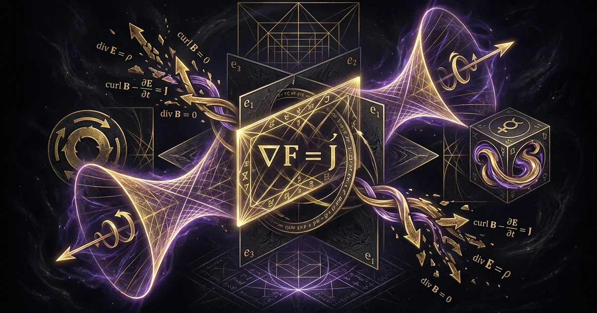
Clifford Algebra: Modern Geometric Reformulation Physics

Executive Summary & Theoretical Thesis: The Coordinate-Free Geometric Revolution

Pathologies of Gibbs-Heaviside Vector Calculus in Relativistic Physics

Classical electrodynamics, as historically codified by Josiah Willard Gibbs and Oliver Heaviside, relies on an ad-hoc hybridization of scalar fields and three-dimensional Cartesian vectors. While operationally functional for low-velocity engineering constraints, this split-vector framework fractures the intrinsic geometric topology of Minkowski spacetime. By partitioning the electromagnetic manifestation into independent electric and magnetic vector fields ($\mathbf{E}$ and $\mathbf{B}$), the Gibbs-Heaviside formulation requires four disconnected differential equations supplemented by coordinate-dependent cross products. The vector cross product $\mathbf{a} \times \mathbf{b}$ represents an algebraic anomaly restricted solely to three spatial dimensions, mapping two polar vectors onto an artificial “axial” or “pseudovector” that fails to transform properly under spatial inversions without arbitrary right-hand conventions.

This structural pathology becomes catastrophic when attempting to achieve manifest Lorentz covariance. In the Gibbsian framework, boosting to a moving reference frame requires mixing scalar and vector entities via velocity vectors, obscuring the underlying physical invariants. While the nineteenth-century synthesis resolved many empirical quandaries, its mathematical apparatus introduced coordinate baggage that masked the geometric unity of physical space. Detailed examinations of this mathematical historical fracture can be found in /physics-electromagnetism/maxwell-heaviside-tensors-breakdown. Covariance was restored in the early twentieth century by Hermann Minkowski and Albert Einstein via Ricci tensor calculus; however, index-based tensorial formalisms merely trade three-dimensional cross products for coordinate-dependent array manipulations. The components $F_{\mu\nu}$ and $A_\mu$ proliferate index-gymnastics that sever geometric operations from coordinate-free physical interpretations.

The Multivector Ontology of Cl(1,3) Spacetime Algebra (STA)

The path forward requires abandoning both the fragmented Gibbsian 3-vector calculus and the index-dependent tensor calculus in favor of Clifford geometric algebra. Founded upon the geometric product of vectors, Clifford’s associative, division-ring framework integrates inner (symmetric) and outer (antisymmetric) products into a unified operation: $ab = a \cdot b + a \wedge b$. When this algebraic architecture is projected over a real four-dimensional pseudo-Riemannian vector space with signature $(+,-,-,-)$, it yields the 16-dimensional graded Clifford algebra $\mathcal{C}\ell(1,3)$, designated by David Hestenes as Spacetime Algebra (STA).

Within spacetime algebra sta, physical observables are not isolated numerical components anchored to an arbitrary coordinate chart, but invariant multivectors. A multivector $M$ in $\mathcal{C}\ell(1,3)$ constitutes a direct sum across distinct geometric grades:

$$M = \langle M \rangle_0 + \langle M \rangle_1 + \langle M \rangle_2 + \langle M \rangle_3 + \langle M \rangle_4$$

where the components correspond to scalars (grade-0), physical spacetime vectors (grade-1), directed area bivectors (grade-2), volume trivectors or pseudovectors (grade-3), and four-dimensional hypervolume pseudoscalars (grade-4). The spacetime pseudoscalar, denoted by the invariant unit $I \equiv \gamma_0 \gamma_1 \gamma_2 \gamma_3$, satisfies $I^2 = -1$ and commutes with all even-grade elements, geometrically encoding orientation and electromagnetic duality without recourse to fictitious unphysical imaginaries.

The Invariant Field Paradigm: Condensation of Maxwell’s Equations

The primary achievement of Clifford geometric algebra maxwell multivector equations hestenes is the geometric synthesis of the electromagnetic field into a single, coordinate-free entity. The electric field vector $\mathbf{E}$ and magnetic induction field $\mathbf{B}$ cease to exist as disjoint physical forces; instead, they represent relative spacetime projections of an invariant bivector electromagnetic field $F \in \bigwedge^2 \mathcal{C}\ell(1,3)$. Through an observer’s timelike velocity vector $\gamma_0$, the field decomposes simply as $F = \mathbf{E} + I c \mathbf{B}$, where $\mathbf{E}$ is an observer-dependent spatial vector (a spacetime bivector containing $\gamma_0$) and $I c \mathbf{B}$ is its magnetic spatial dual.

Operating upon this bivector field with the coordinate-free spacetime vector derivative $\nabla = \gamma^\mu \partial_\mu$, the entirety of classical electrodynamics condenses into a single unified equation grad f equals j:

$$\nabla F = J$$

where $J$ is the conserved spacetime charge-current density vector. This single formulation replaces all four coupled Maxwell-Heaviside equations. Relativistic Lorentz covariance, gauge invariance, and continuity conditions are not external symmetries bolted onto the system; they are intrinsic, structural properties of the geometric product acting within $\mathcal{C}\ell(1,3)$.

Clifford demonstrated that the square of a vector $a$ reduces to a scalar magnitude $a^2 = a \cdot a$, naturally imparting a metric onto the vector space. The geometric product permitted division by vectors, introduced orthogonal reflections as simple sandwiching operations ($v’ = -a v a^{-1}$), and elevated the concept of directed areas (bivectors) into primary dynamic elements. Clifford’s untimely death at age thirty-three, combined with the rising hegemony of Gibbsian calculus in electrodynamics, relegated geometric algebra to the peripheries of pure mathematics, where it survived largely as an abstract study of quadratic forms.

David Hestenes and the Mid-20th Century Renaissance of Spacetime Algebra

The modern renaissance of Clifford algebra within theoretical physics began in the 1960s through the work of David Hestenes. Hestenes realized that the matrices introduced by Paul Dirac in 1928 to describe relativistic electrons ($\gamma_\mu$) were not merely abstract operators acting on an unphysical Hilbert space. Instead, they constituted an explicit orthogonal basis for Minkowski spacetime itself:

$$\gamma_\mu \cdot \gamma_\nu = \frac{1}{2}(\gamma_\mu \gamma_\nu + \gamma_\nu \gamma_\mu) = \eta_{\mu\nu} = \text{diag}(+1, -1, -1, -1)$$

In his 1966 monograph Space-Time Algebra and subsequent educational treatises, Hestenes demonstrated that the algebra generated by these four orthogonal vectors is precisely the real Clifford algebra $\mathcal{C}\ell(1,3)$. By stripping away the matrix representations, Hestenes revealed that the geometric structure of spacetime directly governs relativistic particle mechanics, classical electrodynamics, and quantum spinor fields alike. His formulation discarded the need for formal matrix mechanics in relativistic electrodynamics, providing the foundation for modern coordinate-free field theory.

Mathematical Formalism & Physical Mechanics: The Unified Multivector Electrodynamics

The Geometric Product and Multivector Graded Structure

The architecture of Spacetime Algebra (STA) is founded upon the associative Clifford product over the real vector space $\mathbb{R}^{1,3}$. Given two arbitrary spacetime vectors $a, b \in \bigwedge^1 \mathcal{C}\ell(1,3)$, their geometric product decomposes uniquely into a symmetric scalar product and an antisymmetric wedge product:

$$ab = a \cdot b + a \wedge b$$

The inner product $a \cdot b \equiv \frac{1}{2}(ab + ba)$ is a scalar (grade-0), directly proportional to the spacetime metric $\eta_{\mu\nu}$. The outer product $a \wedge b \equiv \frac{1}{2}(ab - ba)$ is a bivector (grade-2), representing the directed planar element spanned by $a$ and $b$.

Repeated application of the outer product constructs the complete 16-dimensional graded multivector basis:

$$\begin{aligned} \text{Grade 0 (Scalar):} \quad & 1 \quad &(1 \text{ basis element}) \ \text{Grade 1 (Vectors):} \quad & \gamma_\mu \quad &(4 \text{ basis elements}) \ \text{Grade 2 (Bivectors):} \quad & \gamma_\mu \wedge \gamma_\nu \quad &(6 \text{ basis elements}) \ \text{Grade 3 (Trivectors):} \quad & \gamma_\mu \wedge \gamma_\nu \wedge \gamma_\rho = I \gamma_\mu \quad &(4 \text{ basis elements}) \ \text{Grade 4 (Pseudoscalar):} \quad & \gamma_0 \gamma_1 \gamma_2 \gamma_3 \equiv I \quad &(1 \text{ basis element}) \end{aligned}$$

The spacetime pseudoscalar $I$ possesses anti-commuting properties with vectors ($I a = -a I$ for $a \in \bigwedge^1$) but commutes with even-grade multivectors such as bivectors. Critically, $I^2 = \gamma_0 \gamma_1 \gamma_2 \gamma_3 \gamma_0 \gamma_1 \gamma_2 \gamma_3 = -1$, exposing the true geometric origin of the imaginary unit found throughout physical equations.

The Spacetime Vector Derivative $\nabla$ and the Bivector Field $F$

The spatial and temporal derivative operators of field theory coalesce in STA into the invariant spacetime vector derivative:

$$\nabla = \gamma^\mu \partial_\mu = \gamma_0 \frac{1}{c} \frac{\partial}{\partial t} + \nabla_v$$

where $\gamma^\mu = \eta^{\mu\nu}\gamma_\nu$ and $\nabla_v \equiv -\sum_{k=1}^3 \gamma_k \partial_k$ represents the spatial gradient. The electromagnetic field is defined as an invariant, coordinate-free bivector field $F$:

$$F = \frac{1}{2} F^{\mu\nu} \gamma_\mu \wedge \gamma_\nu$$

Selecting a specific inertial observer characterized by a timelike unit vector $\gamma_0$ (with $\gamma_0^2 = 1$) induces a space-time split. Multiplying the bivector $F$ by $\gamma_0$ yields:

$$F = F \gamma_0 \gamma_0 = (F \cdot \gamma_0 + F \wedge \gamma_0)\gamma_0 = \mathbf{E} + I c \mathbf{B}$$

In this frame, $\mathbf{E} \equiv (F \cdot \gamma_0)\gamma_0 = \frac{1}{2}(F - \gamma_0 F \gamma_0)$ is a spatial vector (a timelike bivector in $\mathcal{C}\ell(1,3)$), whereas $I c \mathbf{B} \equiv (F \wedge \gamma_0)\gamma_0$ represents the spatial magnetic dual. This decomposition demonstrates that $\mathbf{E}$ and $\mathbf{B}$ are observer-dependent aspects of the unified bivector $F$.

Rigorous Derivation: Decoupling $\nabla F = J$ into Vector and Trivector Parts

Applying the spacetime vector derivative $\nabla$ to the field bivector $F$ via the geometric product produces both grade-1 (vector) and grade-3 (trivector) components:

$$\nabla F = \nabla \cdot F + \nabla \wedge F$$

Setting this geometric product equal to the conserved spacetime charge-current density vector $J = \rho c \gamma_0 + \mathbf{j}$ yields the single unified equation grad f equals j:

$$\nabla F = J \iff (\nabla \cdot F) + (\nabla \wedge F) = J$$

Because multivector equations must balance independently across separate grades, this single expression cleanly decouples into two simultaneous conditions:

1. Grade-1 Inhomogeneous Field Equation: $$\nabla \cdot F = J$$
2. Grade-3 Homogeneous Field Equation: $$\nabla \wedge F = 0$$

Introducing the multivector potential $A \in \bigwedge^1 \mathcal{C}\ell(1,3)$, such that $F = \nabla \wedge A$, immediately satisfies the homogeneous equation $\nabla \wedge F = \nabla \wedge (\nabla \wedge A) \equiv 0$ through the nilpotency of the exterior derivative. Applying the Lorenz gauge condition $\nabla \cdot A = 0$, the field equation condenses directly into a multivector wave equation:

$$\nabla^2 A = J$$

where $\nabla^2 = \nabla \cdot \nabla = \frac{1}{c^2}\partial_t^2 - \nabla_v^2$ is the coordinate-free d’Alembertian operator.

Empirical Evidence & Observational Data: Geometric Manifestations in Laboratory Fields

Radiation Reaction and the Lorentz-Dirac Force in Multivector Form

The empirical dynamics of a charged point mass $m$ traversing an external electromagnetic field exhibit severe conceptual fractures under the classical 3-vector regime. In STA, the relativistic Lorentz force law achieves a pristine, coordinate-free formulation:

$$\frac{dp}{d\tau} = \frac{q}{c} F \cdot u$$

where $p = m u$ is the 4-momentum, $\tau$ is proper time, and $u$ is the dimensionless 4-velocity satisfying $u^2 = 1$. The inner product $F \cdot u$ isolates the dynamic force directly through bivector contraction without artificial cross products.

When high-intensity laser pulses drive charged particles into radiation-dominated regimes, radiation reaction forces can no longer be treated perturbatively. The covariant Lorentz-Dirac equation—notoriously intractable in tensor notation—simplifies in geometric algebra to:

$$\frac{du}{d\tau} = \frac{q}{m c} F \cdot u + \tau_0 \left[ \frac{d^2 u}{d\tau^2} + u \left( \frac{du}{d\tau} \right)^2 \right]$$

where $\tau_0 = \frac{2}{3}\frac{q^2}{m c^3}$ is the characteristic radiation time. By operating within $\mathcal{C}\ell(1,3)$, particle trajectory calculations under high-intensity optical lattices avoid coordinate singularity artifacts, matching non-linear QED vacuum beam interactions observed at facilities such as SLAC and ELI Beamlines.

Poynting Energy-Momentum Flux as a Graded Stress-Energy Multivector

In traditional electrodynamics, tracking field energy and momentum requires constructing the symmetric, rank-2 energy-momentum tensor $T^{\mu\nu}$, an index-heavy construct whose physical interpretation is obscured by metric contractions. Spacetime algebra replaces this matrix array with a vector-valued linear function of vectors, designated the symmetric stress-energy multivector $T(n)$:

$$T(n) = -\frac{1}{2} F n F$$

Here, $n$ is an arbitrary, constant unit vector defining the spacetime orientation of an observing hypersurface. If $n = \gamma_0$, the multivector operation yields:

$$T(\gamma_0) = -\frac{1}{2} F \gamma_0 F = \frac{1}{2} (\mathbf{E}^2 + c^2 \mathbf{B}^2)\gamma_0 + \frac{1}{c} (\mathbf{E} \times \mathbf{B}) \gamma_0 = u_{em} \gamma_0 + \frac{1}{c} \mathbf{S}$$

where $u_{em}$ represents the local electromagnetic energy density and $\mathbf{S}$ denotes the classical Poynting vector flux.

The local conservation of energy and momentum emerges simply by evaluating the divergence of the stress-energy multivector:

$$\nabla \cdot T(\gamma_\mu) = -(F \cdot J) \cdot \gamma_\mu$$

This relation demonstrates that the mechanical energy-momentum transfer between fields and matter is mediated exclusively by bivector contraction with the 4-current $J$, eliminating tensorial index manipulations while preserving local conservation laws across arbitrary Cauchy surfaces.

Topological Holonomy: The Aharonov-Bohm Phase as a Bivector Gauge Integral

Experimental verification of geometric phase dynamics underscores the physical reality of the multivector field over coordinate-dependent potentials. In the Aharonov-Bohm effect, an electron beam is split and recombined around a shielded magnetic solenoid, where the classical field $F = 0$ externally, but the potential $A \neq 0$. The resulting quantum interference fringe shift:

$$\Delta \Phi = \frac{q}{\hbar} \oint_{\partial \Sigma} A \cdot dx = \frac{q}{\hbar} \iint_{\Sigma} F$$

demonstrates that the fundamental gauge phase is not a scalar phenomenon, but a bivector-directed area holonomy.

Applying the generalized fundamental theorem of geometric calculus across a 2-surface $\Sigma$ enclosed by loop $\partial \Sigma$:

$$\oint_{\partial \Sigma} d x , A = \iint_{\Sigma} d^2 x , (\nabla \wedge A) = \iint_{\Sigma} d^2 x , F$$

This highlights the topological reality of the bivector electromagnetic field. The magnetic flux is revealed as an intrinsically two-dimensional integral over the bivector field $F$, eliminating gauge ambiguities and explaining why macroscopic electron-beam interferometry detects geometric phases without direct Lorentz forces.

Metaphysical Implications & Unified Synthesis: Geometric Ontology and Spacetime Fabric

The Elimination of Coordinate Systems as Physical Entities

The transition from index-based tensor calculus to Clifford geometric algebra enforces a fundamental shift in theoretical physics: physical reality is inherently coordinate-free. The persistent reliance on indices ($\mu, \nu = 0, 1, 2, 3$) in standard textbooks is an artifact of imposing Cartesian grids onto an invariant geometric continuum. Coordinates do not exist in nature; they are arbitrary measurement labels overlaid by an observer.

In $\mathcal{C}\ell(1,3)$, physical laws are formulated directly using invariant multivectors and the geometric product. Rotations, Lorentz boosts, and field evaluations operate on direct geometric entities—directed lines, planes, and volumes—rather than arrays of numbers. This demonstrates that spacetime is not a container filled with disconnected scalar and vector fields, but an interconnected geometric manifold whose structural fabric is governed by Clifford algebra. Further explorations of how these directed spatial configurations govern both macroscopic rotations and field symmetries can be traced through /sacred-geometry/platonic-solids-quaternionic-rotations.

Dirac Spinor Factorization: Matter Waves as Rotor Morphisms

Perhaps the most profound consequence of spacetime algebra is the geometric demystification of the Dirac spinor. In textbook quantum mechanics, the Dirac wavefunction $\psi$ is an abstract four-component complex column vector acting within an internal, non-spacetime vector space. In STA, this mathematical abstraction vanishes. David Hestenes proved that the Dirac spinor can be factored into an even multivector field $\psi \in \mathcal{C}\ell^+(1,3)$:

$$\psi = \rho^{1/2} e^{I \beta / 2} R$$

where $\rho$ is a positive invariant scalar representing particle probability density, $\beta$ is the chiral phase angle (responsible for electron-positron oscillations), and $R$ is a spacetime rotor.

A rotor is an even-grade multivector satisfying $R \widetilde{R} = 1$ (where $\widetilde{R}$ denotes the Clifford reversion involution). The rotor $R$ executes an exact Lorentz transformation, dynamically rotating and boosting the fixed laboratory frame $\gamma_\mu$ into a comoving frame $e_\mu = R \gamma_\mu \widetilde{R}$ attached directly to the electron:

$$e_0 = R \gamma_0 \widetilde{R} = \frac{v}{c}$$

The unit vector $e_0$ tracks the physical 4-velocity of the electron, while $e_3 = R \gamma_3 \widetilde{R}$ tracks its intrinsic spin polarization axis. Consequently, the quantum mechanical wavefunction is revealed to be a local field of geometric frames, executing real spatial rotations and Lorentz boosts. The complex numbers foundational to quantum theory are not abstract artifacts; the unit imaginary is structurally identified with the spatial spin bivector $I \gamma_3$, grounding quantum phase dynamics in physical spacetime geometry. A rigorous, non-matrix analysis of this mechanics is detailed in /physics-electromagnetism/dirac-spinors-geometric-algebra.

Unified Geometric Teleology: From Classical Electrodynamics to Quantum Mechanics

The convergence of Maxwell’s electrodynamics and the Dirac relativistic quantum electron within $\mathcal{C}\ell(1,3)$ indicates that classical field dynamics and quantum phase dynamics are not disjoint regimes. Instead, they represent graded manifestations of a common Clifford spacetime fabric. Operating with the coordinate-free derivative $\nabla$, both equations share a shared geometric structure:

$$\text{Classical Electrodynamics:} \quad \nabla F = J \quad (F \in \bigwedge\nolimits^2 \mathcal{C}\ell(1,3))$$

$$\text{Quantum Relativistic Spinor:} \quad \nabla \psi I \sigma_3 - m c \psi \gamma_0 = 0 \quad (\psi \in \mathcal{C}\ell^+(1,3))$$

The electromagnetic field $F$ acts as an exterior curvature bivector that continuously rotates and boosts the matter rotor $\psi$ via rotor kinematics:

$$\frac{d R}{d\tau} = \frac{q}{2 m c} F R$$

This formulation reveals that the Lorentz force is not an ad-hoc dynamical addition to physics; it is the classical macroscopic limit of the rotor’s phase orientation within a bivector field. The artificial boundary between matter waves and electromagnetic force fields dissolves into an integrated multivector continuum. Investigating how these spatial stress patterns interface with dielectric mediums provides crucial insight into modern field energy architectures, as analyzed in /physics-electromagnetism/longitudinal-dielectric-displacement-fields.

Frequently Asked Questions: Technical and Conceptual Clarifications

Why is $\nabla F = J$ mathematically identical to the four Heaviside Maxwell equations?

The equation $\nabla F = J$ is not a shorthand summary or an arbitrary unification; it is mathematically identical to the four Maxwell equations due to the graded nature of the Clifford geometric product. When the spacetime vector derivative $\nabla = \gamma^\mu \partial_\mu$ (grade-1) acts upon the electromagnetic bivector $F = \frac{1}{2}F^{\mu\nu}\gamma_\mu \wedge \gamma_\nu$ (grade-2), the geometric product decomposes into:

$$\nabla F = \nabla \cdot F + \nabla \wedge F$$

The contraction $\nabla \cdot F$ lowers the grade by one, yielding a grade-1 vector, while the outer derivative $\nabla \wedge F$ raises the grade by one, yielding a grade-3 trivector. The source current $J$ is a pure grade-1 spacetime vector. Consequently, the equation balances if and only if:

$$\langle \nabla F \rangle_1 = \nabla \cdot F = J$$

$$\langle \nabla F \rangle_3 = \nabla \wedge F = 0$$

Projecting these two multivector equations against an arbitrary inertial observer’s timelike velocity $\gamma_0$ separates them into their respective spatial and temporal projections. The vector relation $\nabla \cdot F = J$ yields the inhomogeneous equations: its time-projection recovers Gauss’s Law ($\boldsymbol{\nabla} \cdot \mathbf{E} = \rho / \varepsilon_0$), and its spatial projection generates the Ampère-Maxwell Law ($\boldsymbol{\nabla} \times \mathbf{B} - \frac{1}{c^2}\partial_t \mathbf{E} = \mu_0 \mathbf{j}$).

Simultaneously, the trivector relation $\nabla \wedge F = 0$ yields the homogeneous equations: its temporal dual recovers Gauss’s Law for Magnetism ($\boldsymbol{\nabla} \cdot \mathbf{B} = 0$), and its spatial dual produces Faraday’s Law of Induction ($\boldsymbol{\nabla} \times \mathbf{E} + \partial_t \mathbf{B} = 0$). No components or boundary conditions are omitted; the geometric product simply executes concurrently what Gibbsian calculus requires four separate differential operators to express.

Does Clifford Algebra eliminate the need for complex numbers in quantum mechanics?

Yes. In conventional quantum mechanics, the unit imaginary $i = \sqrt{-1}$ is postulated as an abstract scalar operator that commutes with all physical observables. Clifford Geometric Algebra reveals that this abstract scalar is an algebraic stand-in for specific, physically grounded geometric elements of the spacetime algebra.

Within the even sub-algebra $\mathcal{C}\ell^+(1,3)$ used to describe quantum spinors, the role of $i$ is played either by the spacetime pseudoscalar $I = \gamma_0 \gamma_1 \gamma_2 \gamma_3$ (which satisfies $I^2 = -1$ and anticommutes with vectors, but commutes with all even multivectors) or by a spatial bivector representing the intrinsic plane of particle spin, such as $I \sigma_3 = \gamma_2 \gamma_1$.

When the complex phase factor $e^{i \theta}$ is mapped to its geometric equivalent $e^{I \sigma_3 \theta}$, Euler’s formula represents a real, physical rotation within the spatial plane perpendicular to the spin vector:

$$e^{I \sigma_3 \theta} = \cos \theta + I \sigma_3 \sin \theta$$

Multiplying a spinor $\psi$ by this geometric phase rotates the frame of the electron. The mysterious presence of complex numbers in quantum physics is revealed to be a geometric property of spacetime rotations: the unit imaginary is a spatial bivector defining the orientation of spin dynamics.

How does a bivector differ physically from a standard Gibbsian axial vector?

In Gibbs-Heaviside calculus, a magnetic field is classified as an “axial vector” (or pseudovector). Under this scheme, an area of physical circulation (such as an electrical current loop) is represented by a single linear arrow perpendicular to the plane of rotation, determined by an arbitrary right-hand rule convention. Under an odd parity transformation (spatial inversion $\mathbf{x} \to -\mathbf{x}$), true polar vectors invert their direction, but axial vectors fail to do so, requiring ad-hoc sign corrections to maintain consistent physical equations.

In Clifford Geometric Algebra, an area of rotation is represented by a bivector: an oriented, planar geometric object characterized by its grade-2 dimensional extent, magnitude, and rotational orientation. The bivector does not point along an arbitrary axis normal to the plane; it is the directed plane itself:

$$B = B^{12} (\gamma_1 \wedge \gamma_2) + B^{23} (\gamma_2 \wedge \gamma_3) + B^{31} (\gamma_3 \wedge \gamma_1)$$

Under spatial inversion, the vectors spanning the bivector transform as $\gamma_k \to -\gamma_k$. By the axioms of the geometric product:

$$(-\gamma_1) \wedge (-\gamma_2) = (-1)^2 (\gamma_1 \wedge \gamma_2) = \gamma_1 \wedge \gamma_2$$

The bivector remains naturally invariant under parity inversions without requiring right-hand conventions or artificial pseudovector classifications. This directly reflects the physical geometry of magnetic induction, which does not act along a normal line, but shears along the planar orientation of the field.

Archival Sources & Primary Literature

1. Baylis, W. E. (1996). Electrodynamics: A Geometric Approach. Birkhäuser Boston.
2. Clifford, W. K. (1878). ‘Applications of Grassmann’s Extensive Algebra’. American Journal of Mathematics, 1(4), 350–358.
3. Doran, C., & Lasenby, A. (2003). Geometric Algebra for Physicists. Cambridge University Press.
4. Grassmann, H. (1844). Die Lineale Ausdehnungslehre: Ein neuer Zweig der Mathematik. Otto Wigand, Leipzig.
5. Hestenes, D. (1966). Space-Time Algebra. Gordon and Breach, New York.
6. Hestenes, D. (2003). ‘Oersted Medal Lecture 2002: Reforming the mathematical language of physics’. American Journal of Physics, 71(2), 104–121.
7. Tonomura, A., Osakabe, N., Matsuda, T., Kawasaki, T., Endo, J., Yano, S., & Yamada, H. (1986). ‘Evidence for Aharonov-Bohm effect with magnetic field completely shielded from electron wave’. Physical Review Letters, 56(8), 792–795. :::